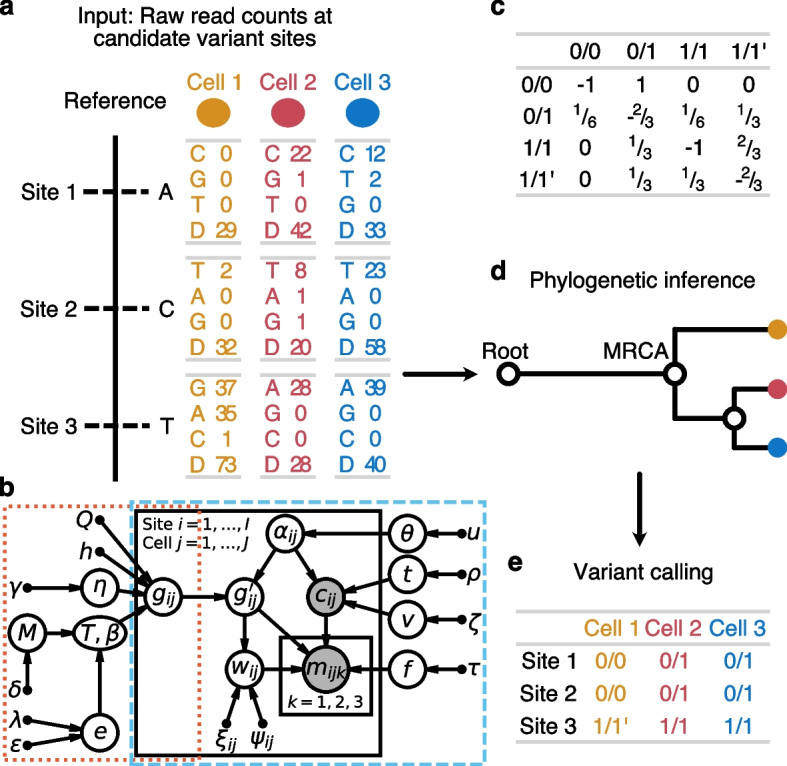
Fig. 1.

Overview of the SIEVE model. a Input data to SIEVE at candidate SNV sites. For a specific cell at an SNV site, fed to SIEVE are the read counts for all nucleotides: reads of the three alternative nucleotides with values in descending order and the total coverage (denoted by D in a). b Graphical representation of the SIEVE model. Bridged by $g_{\mathit{ij}}$, the genotype for site i in cell j, the orange dotted frame encloses the statistical phylogenetic model, and the blue dashed frame highlights the model of raw read counts. Shaded circle nodes represent observed variables, while unshaded circle nodes represent hidden random variables. Small filled circles correspond to fixed hyper parameters. Arrows denote local conditional probability distributions of child nodes given parent nodes. The sequencing coverage $c_{\mathit{ij}}$ follows a negative binomial distribution parameterised by the number of sequenced alleles ${\alpha }_{\mathit{ij}}$, the mean of allelic coverage t and the variance of allelic coverage v. ${\alpha }_{\mathit{ij}}$ is a hidden categorical variable parameterised by ADO rate $\theta$, which has a uniform prior with fixed hyper parameter u. t also has a uniform prior with fixed parameter $\rho$, while v has an exponential prior parameterised by $\zeta$. The nucleotide read counts ${\mathit{m}}_{\mathit{ij}}$ given $c_{\mathit{ij}}$ follow a Dirichlet-multinomial distribution parameterised by ADO-affected genotype $g_{\mathit{ij}}^{\prime }$, which is a hidden random variable depending on ${\alpha }_{\mathit{ij}}$ and genotype $g_{\mathit{ij}}$, effective sequencing error rate f, which has en exponential prior with fixed hyper parameter $\tau$, and overdispersion $w_{\mathit{ij}}$, which is a hidden categorical variable dependent on $g_{\mathit{ij}}^{\prime }$ parameterised by fixed parameters ${\xi }_{\mathit{ij}}$ and ${\psi }_{\mathit{ij}}$ for each category. $g_{\mathit{ij}}$ is determined by the statistical phylogenetic model parameterised by fixed rate matrix Q, fixed number of categories h as well as shape parameter $\eta$ with exponential prior for site-wise substitution rates, and tree topology $\mathcal{T}$ along with branch lengths $\mathit{\beta }$. $\mathcal{T}$ and $\mathit{\beta }$ have a coalescent prior with an exponentially growing population parameterised by effective population size M, which has a multiplicative inverse prior, and growth rate e, which has a laplace prior parameterised by $\lambda$ and $ϵ$. c The transition rate matrix in the statistical phylogenetic model. During an infinitesimal time interval only one change is allowed to occur. d The cell phylogeny inferred from the data with SIEVE. Not only is the tree topology crucial, but also the branch lengths. The root represents a normal cell, and the only direct child of the root is the most recent common ancestor (MRCA) of all cells. e Variant calling given the inferred cell phylogeny. For further details, see the “Methods” section