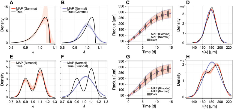
Fig 5. Inference and prediction where parameter distribution is misspecified.
We explore a case where the underlying growth rate distribution has (A–C) a skewed distribution with (μλ, σλ, ωλ) = (1, 0.05, −1.5), and (e–g) a bimodal distribution, modelled as the mixture wλ1 + (1 − w)λ2 with , and w = 0.4. To ensure identifiability, we use a large sample size of N = 1000 per time point. In (A,E) the true form of the growth rate distribution is used, whereas in (B,F) the growth rate distribution is misspecified and assumed to be normal. Shaded regions in (A,B,E,F) indicate 95% credible intervals for the density. In (C,G), predictions at the MAP estimates (equivalent to MLE) are compared to the data. A 95% prediction interval is shown for the true model (shaded) and the misspecified model (blue dashed), solid curves to the mean, and violin plots show the data. In (D,H), we compare predictions for the density from the true and misspecified models at t = 4.

