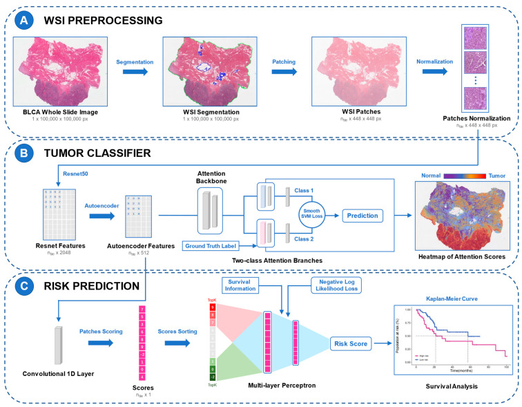
Figure 1.

Study flow chart and the layouts of the DL models. The framework of BlcaMIL is shown in A and B and the framework of MibcMLP is shown in A and C. (A) Each WSI was first segmented into tissue-containing regions (green border) and empty regions inside the tissue (blue border), and then patches with 448 × 448 pixels were generated. (B) Feature extraction was performed on all patches using ResNet-50, and dimensionality reduction was performed with Autoencoder. Through the MIL model with attention mechanism, the extracted patch-level features were input into the BlcaMIL model, the attention scores of these patches were output, and the average pooling function was used to aggregate them into the WSI-level to make the final diagnosis. Heatmaps visualize ROIs for the model. (C) Patch-level features were fed into the network along with survival information, and each patch was assigned a risk score through an iterative learning process. Then, the 50 patches with the highest and lowest scores were selected to be input to the MLP model to predict patient survival. Finally, MIBC patients were stratified using the resulting risk scores. DL, deep learning; WSI, whole slide image; MIL, multiple instance learning; ROI, region of interest; MLP, multi-layer perceptron; MIBC, muscle invasive bladder cancer.