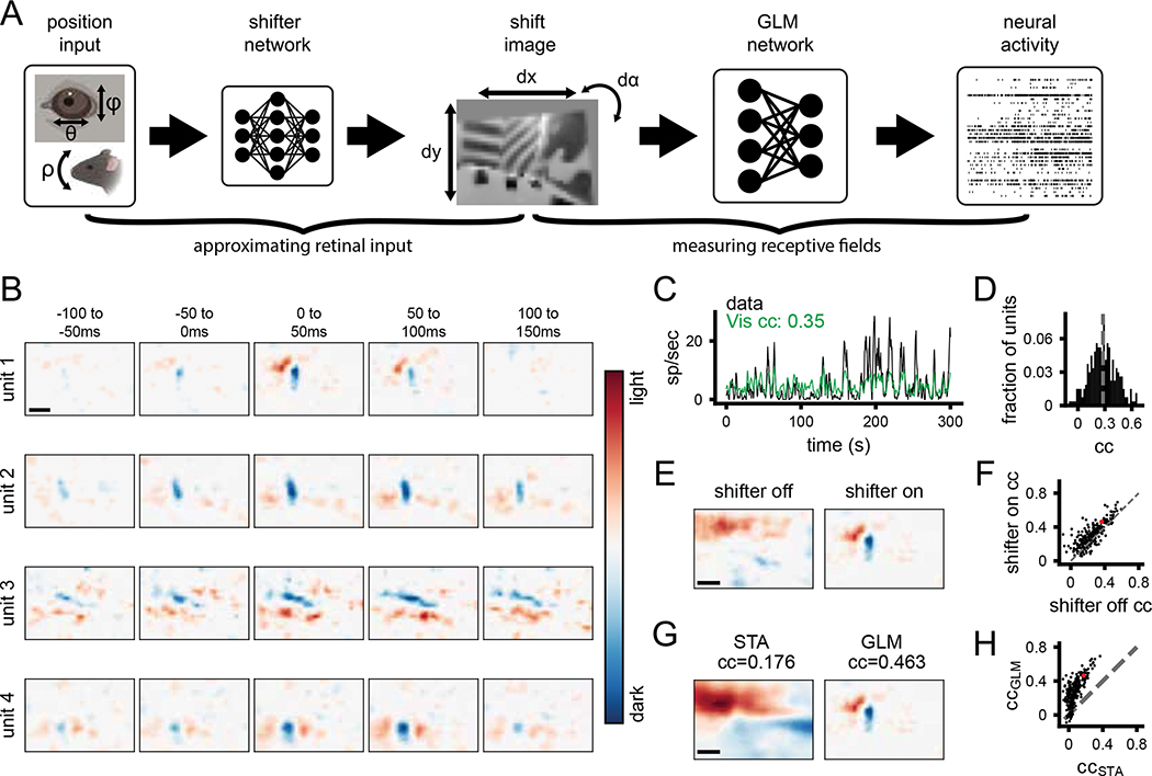
Figure 2: A generalized linear model accurately estimates spatiotemporal receptive fields during free movement.
A) Schematic of processing pipeline. Visual and positional information is used as input into the shifter network, which outputs parameters for an affine transformation of the world-camera image. The transformed image frame is then used as the input to the GLM network to predict neural activity. B) Four example freely moving spatiotemporal visual receptive fields. Scale bar for RFs represents 10 degrees. C) Example actual and predicted smoothed (2 s window) firing rates for unit 3 in B. D) Histogram of correlation coefficients (cc) for the population of units recorded. Average cc shown as gray dashed line. E) Example of a freely moving RF with the shifter network off (left) and on (right) at time lag 0 ms. Colormap same as B. F) Scatter plot showing cc of predicted versus actual firing rate for all units with the shifter network off vs on. Red point is the unit shown in E. G) Example receptive field calculated via STA (left) versus GLM (right). H) Scatter plot showing cc of predicted vs actual firing rate for all units, as calculated from STA or GLM. Red point is the unit shown in G.

