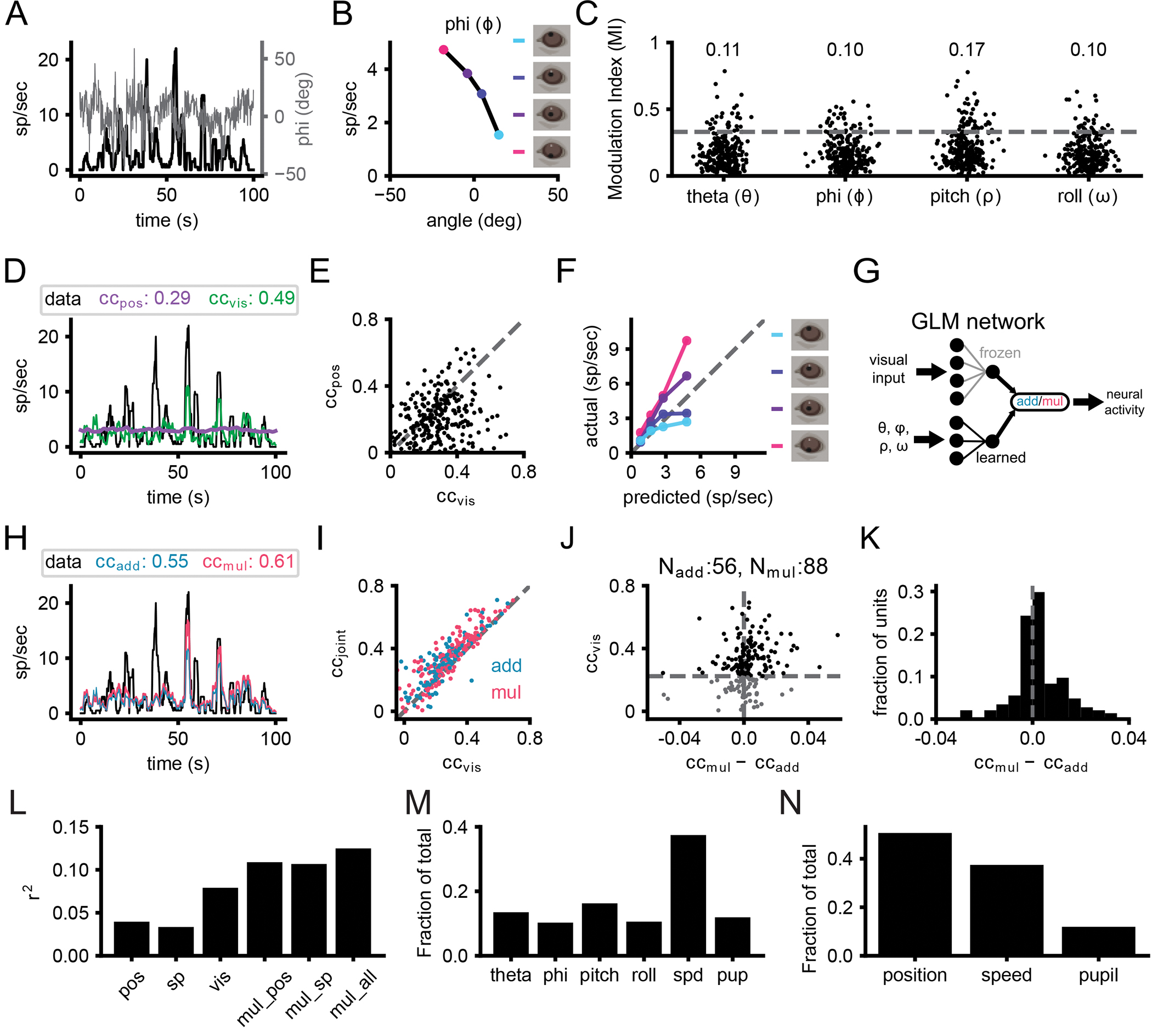
Figure 4: V1 neurons integrate visual and position signals.

A) Overlay of vertical eye angle (phi; gray) and the smoothed firing rate of an example unit (black). B) Example tuning curve for head pitch. Colored points denote the quartiles of phi corresponding to panel F. C) Scatter of the modulation indices for eye position and head orientation (N=268 units, 4 animals). Numbers at top of the plot represent the fraction of units with significant tuning. D) Same unit as A. Example trace of smoothed firing rates from neural recordings and predictions from position-only and visual-only fits. E) Scatter plot of cc for position-only and visual-only fits for all units. F) Gain curve for the same unit in A and C. Modulation of the actual firing rates based on phi indicated by color. G) Schematic of joint visual and position input training. H) Same unit as A, C, and E. Smoothed traces of the firing rates from the data, additive and multiplicative fits. I) Correlation coefficient for visual-only versus joint fits. Each point is one unit, color coded for the joint fit that performed best. J) Comparison of additive and multiplicative fits for each unit. Units characterized as multiplicative are to the right of the vertical dashed line, while additive ones are to the left. Horizontal dashed line represents threshold set for the visual fit, since in the absence of a predictive visual fit, a multiplicative modulation will be similar to an additive modulation. K) Histogram of the difference in cc between additive and multiplicative models. The visual threshold from I was applied to the data. L) Explained variance (r²) for position only (pos), speed and pupil only (sp), visual only (vis), multiplicative with eye/head position (mul_pos), multiplicative with speed and pupil (mul_sp), and multiplicative with eye/head position, speed and pupil (mul_all). M) The fraction of contribution of the weights for multiplicative fits with eye/head position, speed (spd) and pupil (pup). N) Same as M but summing together the contribution for eye/head position.