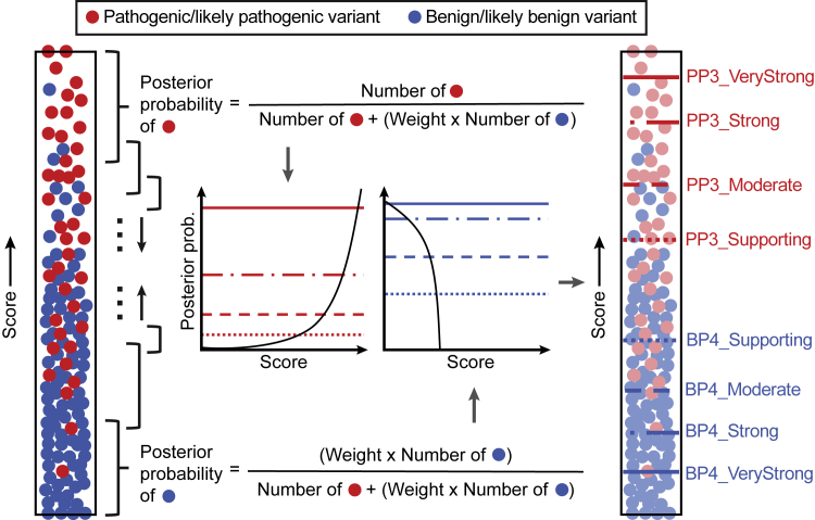
Figure 2.
Conceptual representation of the estimation of intervals for evidential support
An example in silico tool that is supposed to assign higher scores to pathogenic variants is shown. Each filled circle represents a variant, either pathogenic/likely pathogenic (red) or benign/likely benign (blue) as recorded in the ClinVar 2019 set. All unique scores were first sorted and each score was then set as the center of the sliding window or the local interval (black-colored braces), within which posterior probabilities were calculated. Here, to ensure that a sufficient number of variants were included in each local interval, was adaptively selected to be the smallest value so that the interval around a prediction score s incorporated at least 100 pathogenic and benign variants (combined) from the ClinVar 2019 set and at least 3% of rare variants from the gnomAD set with predictions in the given local interval, separately for each method (technically, is a function of score s for each predictor). These numbers were proportionally scaled at the ends of the score range. The estimated posterior probabilities were then plotted against the output scores. Using posterior probability thresholds defined in Table 1, score thresholds were subsequently obtained for pathogenicity (PP3) and benignity (BP4) for each method. Here, the number of benign variants was weighted to calibrate methods according to the prior probability of pathogenicity. The weight was calculated by dividing the ratio of pathogenic and benign variant counts in the full data set by the prior odds of pathogenicity; see Equation 3. The pathogenic and benign counts (and this weight) slightly varied for each method because scores were not available for all variants in the data set for some tools. In this study, the estimated prior probability of pathogenicity (0.0441) was used to account for the enrichment of pathogenic/likely pathogenic variants in ClinVar. The estimated prior probability of benignity was assumed to be 1–0.0441 = 0.9559.

