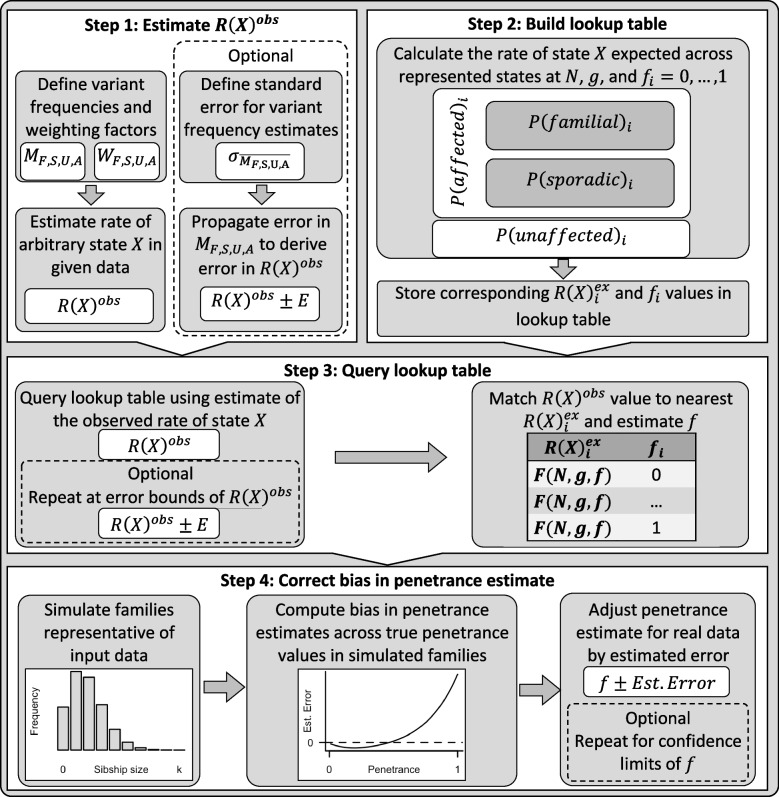
Fig. 1.

Summary of the key steps within this penetrance estimation approach. Legend: Step 1: Variant frequencies (M) and weighting factors (W) are defined for a valid subset of the familial (F), sporadic (S), unaffected (U), and affected (A) states (see Table 1) to calculate rate of one of these states, arbitrarily labelled state X, among families harbouring the pathogenic variant across those states with data provided, $R{\left(X\right)}^{\mathit{obs}}$. Step 2: Eqs. (5–8) are applied to calculate $P(familial)$, $P(sporadic)$, $P(unaffected)$, and $P(affected)$, for a series of penetrance values, $f_i=0,\cdots ,1$, at a defined sibship size, $N$, and with disease risk $g$ for people not harbouring the variant. The rate of state X expected at each $f_i$ among variant harbouring families from those states represented in Step 1, $R{\left(X\right)}_i^{\mathit{ex}}$, is calculated and stored alongside the corresponding $f_i$ in a lookup table. Step 3: The lookup table is queried using $R{\left(X\right)}^{\mathit{obs}}$ to identify the closest $R{\left(X\right)}_i^{\mathit{ex}}$ value and corresponding $f_i$. Step 4: Bias in the obtained $f_i$ estimate is corrected by simulating a population of families representative of the sample data, estimating the difference between true and estimated penetrance values in this population between $f=0,\cdots ,1$ and adjusting the estimated $f_i$ by error predicted within a polynomial regression model fitted upon the simulated estimate errors. Optional step: Confidence intervals for $R{\left(X\right)}^{\mathit{obs}}$ can be calculated from error in the estimates of $M$ provided [48]; Penetrance is estimated as in Steps 3 and 4 for the interval bounds. All steps within this approach are comprehensively detailed in Additional File: Sect. 1.1