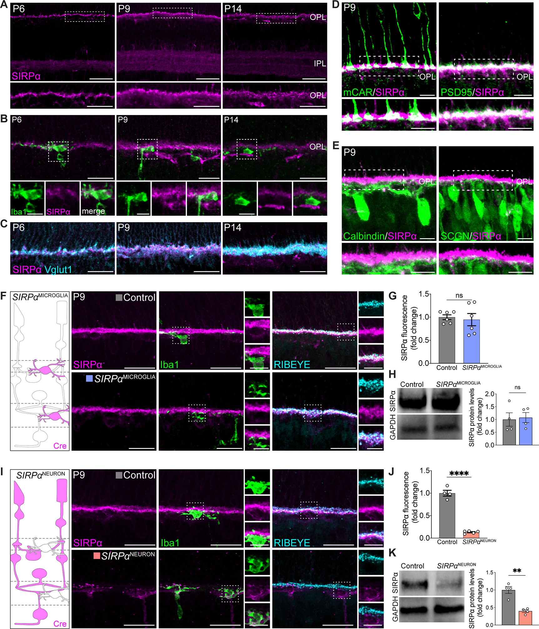
Figure 2. Neuronal SIRPα was enriched during periods of peak microglia phagocytosis.

(A) Representative images showing P6, P9, and P14 WT SIRPα staining (magenta) in the synaptic layers. Scale bars, 50 μm (top) and 25 μm (bottom). See also Figure S2A–B.

(B) Representative images showing little SIRPα signal in Iba1⁺ microglia (green). Scale bars, 25 μm and 10 μm (insets). See also Figure S2C.

(C) Representative images showing colocalization of SIRPα (magenta) and Vglut1⁺ photoreceptor terminals (cyan) in the OPL. Scale bars, 25 μm. See also Figure S2C.

(D) Representative images showing colocalization of SIRPα (magenta) with cone (mCAR) and rod (PSD95) terminals (green). Scale bars, 10 μm. See also Figure S2D.

(E) Representative images showing SIRPα (magenta) with horizontal cell (Calbindin) and cone bipolar cell (SCGN) terminals (green). Scale bars, 10 μm. See also Figure S2D.

(F) Schematic of microglial SIRPα deficiency model (SIRPα^MICROGLIA). Example images showing staining of SIRPα (magenta), microglia (Iba1, green), and OPL synapses (RIBEYE, cyan) in this model at P9. Scale bars, 25 μm and 10 μm (insets). See also Figure S2F.

(G) Levels of SIRPα fluorescence in OPL in SIRPα^MICROGLIA relative to controls, n=6 per group. Data were compared using an unpaired t-test.

(H) Representative immunoblot image and quantification of SIRPα in whole retina from P9 WT and SIRPα^MICROGLIA mice. n=3 per group. Data were compared using an unpaired t-test.

(I) Schematic of neuronal SIRPα deficiency model (SIRPα^NEURON). Example images showing staining of SIRPα (magenta), microglia (Iba1, green), and OPL synapses (RIBEYE, cyan) in this model at P9. Scale bars, 25 μm and 10 μm (insets). See Figure S2F.

(J) Levels of SIRPα fluorescence in OPL in SIRPα^NEURON mice relative to controls, n=4 control and 5 SIRPα^NEURON. Data were compared using an unpaired t-test.

(K) Representative immunoblot image and quantification of SIRPα in whole retina from P9 WT and SIRPα^NEURON. n=3 per group. Data were compared using an unpaired t-test.

Data from (H) and (K) were obtained from one experiment. (G) and (J) were pooled from two independent experiments. All data are presented as the mean ± SEM. **p<0.01, ****p<0.0001, ns, not significant. See also Figures S2–3.