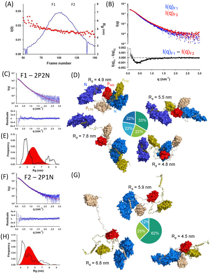
Figure 7.
SEC-SAXS of N∆230−PFL complex. (A) SEC-SAXS elution profile and Rg across the elution peak; 50 μL of N∆230−PFL sample were injected onto a Superdex 200 column and monitored on-line by SAXS. The blue line shows the intensity at zero angle (I0), which is proportional to both MM and concentration. The red dots indicate the values of the radius of gyration calculated from the Guinier approximation at the different time intervals. The shaded areas (labeled F1 and F2) show the frames that were averaged and used for analysis in the next panels. (B) Average SAXS profiles at two different positions in the SEC profile. The upper part shows the curves obtained by averaging the individual profiles recorded across the two fractions (F1 and F2) of the SEC elution peak shown in Panel (A). The lower part shows the difference scattering profile (I(q)F1–I(q)F2). (C) Conformational ensemble modeling by the ensemble optimization method (EOM). The upper panel show the experimental F1scattering profile (blue circles) The red line shows back-calculated scattering curve for a selected ensemble of 4 2P−2N conformers shown in panel (E) (χ2 = 1.95). The lower panel shows the plot of the residuals (blue circles). (D) Representative ensemble of conformers that reproduce the curve at position F1. The pie chart indicates the fraction of each conformer used in the calculated curve. The dimerization domain of P (PMD) is shown in surface representation in red. The rest of the chains of P are shown in wheat and olive and the C-terminal domains (PCTD) are shown in surface representation, while the intrinsically disordered regions are shown as cartoons. The N0 molecules are shown in two shades of blue in surface representation. (E) Rg distribution. The red area shows the Rg distribution calculated for the initial ensemble of conformers (2P−2N), whereas the black line shows the Rg distribution of the selected ensembles that fit the experimental SAXS data (panel (C)). (F) Conformational ensemble modeling by the ensemble optimization method (EOM). The upper panel show the experimental F1 scattering profile (blue circles) The red line shows back-calculated scattering curve for a selected ensemble of three 2P−1N conformers shown in panel H (χ2 = 1.99). The lower panel shows the plot of the residuals (blue circles). (G) Representative ensemble of conformers that reproduce the curve at position F2. The pie chart indicates the fraction of each conformer used in the calculated curve. The P protein is shown as in panel E and the N0 molecule is shown in blue in surface representation. (H) Rg distribution. The red area shows the Rg distribution calculated for the initial ensemble of conformers (2P−1N), whereas the black line shows the Rg distribution of the selected ensembles that fit the experimental SAXS data (panel (F)).

