Prediction and verification of glycosyltransferase activity by bioinformatics analysis and protein engineering

Summary

A significant number of proteins are annotated as functionally uncharacterized proteins. Within this protocol, we describe how to use protein family multiple sequence alignments and structural bioinformatics resources to design loss-of-function mutations of previously uncharacterized proteins within the glycosyltransferase family. We detail approaches to determine target protein active sites using three-dimensional modeling. We generate active site mutants and quantify any changes in enzymatic function by a glycosyltransferase assay. With modifications, this protocol could be applied to other metal-dependent enzymes.

For complete details on the use and execution of this protocol, please refer to Ilina et al. (2022).¹

Graphical abstract

Highlights

• •Bioinformatics workflow to resolve glycosyltransferase structures
• •Three-dimensional modeling to predict active site residues
• •Cloning strategy to generate active site mutant proteins
• •Quantitative glycosyltransferase assay for assessing enzymatic activity

Publisher’s note: Undertaking any experimental protocol requires adherence to local institutional guidelines for laboratory safety and ethics.

A significant number of proteins are annotated as functionally uncharacterized proteins. Within this protocol, we describe how to use protein family multiple sequence alignments and structural bioinformatics resources to design loss-of-function mutations of previously uncharacterized proteins within the glycosyltransferase family. We detail approaches to determine target protein active sites using three-dimensional modeling. We generate active site mutants and quantify any changes in enzymatic function by a glycosyltransferase assay. With modifications, this protocol could be applied to other metal-dependent enzymes.

Before you begin

The protocol describes in silico sequence analyses, 3D-structure modeling, mutational design and protein engineering steps that can be used to design loss-of-function mutants of glycosyltransferases to ultimately validate them in vitro. Outcomes of major steps 1–3 form the basis for producing rationally designed active site mutants in the laboratory (major steps 4 and 5) whose intended (negative) impact on catalysis can be verified as it is described in major step 6. As reported in Ilina et al.,¹ the resulting mutants ultimately served as tools to demonstrate a link between catalytic glycosyltransferase activity of GLT8D1 and cell migratory properties in glioblastoma (by procedures not included in this protocol).

The procedures detailed in this protocol should be adaptable to any other metal-dependent family within the diverse GT-A superfamily of glycosyltransferases and facilitate reproducing the mutant production and validation for GLT8D1 as reported.¹ Moreover, its strategic framework and various key resources are transferable to unrelated cases in principle, and its step-by-step sequence potentially serve as guidance for developing similar protocols for other enzymes with similar metal-dependence. Loss-of-function mutants are informative and affordable laboratory tools in practice, a.o. for elucidating the impact of hypothetical enzyme functions of new target proteins in their respective biological contexts. Here, we describe a practical route to produce them and other informative items as “by-products” (Figure 1). This inter-disciplinary protocol is described a priori for execution by either a multi-disciplinary team, or a single person with training and prior practical experience in protein biochemistry and/or molecular biology as well as protein structural bioinformatics on other projects.

Note: Several steps in major steps 1–3 could be replaced by short-cuts, e.g., through fully-automated computational modeling pipelines. We point this out as Alternatives below but do not discuss it in detail. Many “one-stop shop” methods and interfaces exist, and new improved ones become available continually after being tested on large data sets for general accuracy across varied protein targets.² For some applications and targets, we nonetheless prefer to execute the steps as we described them here in order to quickly recognize (and correct) rare mistakes if they occur, build trust in the outcomes of each part for each particular target, and perhaps also notice peculiarities that lead to further research in the process. This protocol therefore includes steps in which one interacts with the data, e.g., in qualitative consistency checks, while keeping in mind that the intended primary use of these items here is to support laboratory applications in protein engineering as described in major steps 4–6, and similar. By structuring this protocol in six parts, we leave room to its users to swap out methodology in some of them if they wish, and rejoin the protocol later.

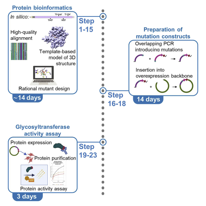
Figure 1.

Schematic illustration of analysis described in major steps 1–4 (steps 1–15)

Collect target protein information online

Timing: ∼1–3 days (repeat occasionally)

• 1.
  Collect information about the target protein’s structural and functional characteristics.

  • a.
    Literature reports about the target protein (if available) should be complemented with annotation available in dynamic online databases. For example, we regularly check: UniProt,³ GeneCards, neXtprot for predicted or known domain architecture, functional features.
  • b.
    These websites also specify if a 3D-structure has been solved and deposited in the Protein Data Bank (PDB).⁴
• 2.Re-check the information that is accessible about your protein periodically during your research project, in intervals of 2–3 weeks.
• 3.Depending on the target and its hypothesized catalytic function, additionally consult more specialized literature relating to that function and/or enzyme-specific online resources (e.g., BRENDA)⁵.
• 4.Since rational design of active site mutations builds on defined or speculative catalytic roles of individual active site residues, gain an overview of a target’s potential mechanistic and biochemical properties through records for characterized enzymes that catalyze similar reactions (if any are known), including substrate specificity.

Note: Consider searching for online information using the human ortholog of your target because often human genes/proteins are the most richly annotated. Some resources may require using its HGNC (HUGO Gene Nomenclature Committee) gene name (e.g., GLT8D1) although most comprehensive resources accept synonyms (e.g., its UniProt identifier GL8D1_HUMAN).

Note: Keep in mind that “annotation” in online resources may be computational and/or predicted through high-throughput methods without follow-up, i.e., hypothetical, and that individual records are updated dynamically.

Select and install software as needed

Timing: ∼1–2 days

Most in silico steps in this protocol (see Figure 1) can be executed using online resources (i.e., web servers that run software server-side according to your instructions, and return the results interactively or by email). In a few instances we recommend using local software installations (Table 1).

• 5.
  Before you begin, select and install software as needed, to facilitate:

  • a.
    Protein 3D-structure visual inspection (e.g., UCSF Chimera⁶).
  • b.
    Multiple sequence alignment (MSA) viewing and editing (e.g., ClustalX⁷ or Jalview⁸).
  • c.
    Other steps that you may prefer running locally, over running them online.

Note: To run the locally used programs mentioned here, a typical personal computer will suffice (see suggestions in the key resources table).

Note: Familiarize yourself well with programs that you have not yet used often. Tutorials are usually available via their download websites (Table 1). For further background information please refer to the literature (see suggestions in Table 2).

CRITICAL: Please respect licensing, citation and feedback requirements when using third party software online or locally.

CRITICAL: Archive a copy of the software version(s) that you used in order to ensure reproducibility and to reply to peer-reviewers’ requests at a later time. Not all software download sites offer old versions. A computer with a compatible operating system version will also be needed for this purpose.

Note: We advise against using local installations of programs that use extensive or specialist databases in their execution (e.g., HHpred,⁹SWISS-MODEL¹⁰). Instead, their online implementations assure frequent updates of the associated databases and interactive result displays. To account for the dynamic nature of these resources in research reporting, analysis dates must always be included with results from web servers that depend on dynamically updated databases. Maintaining these databases locally is not worth the effort unless you require extreme data privacy that precludes submitting requests to extramural web servers.

Note: Although this is beyond the scope of this protocol, generating high-quality scientific images for publication might be another important consideration influencing your software preferences. Locally installed software often proves superior, more versatile and/or less time-consuming for this purpose, compared with online options. For example, UCSF Chimera is one of many excellent programs that are available for visualizing and manipulating protein 3D-structures effectively that also produce high-resolution molecular graphics.

Table 1.

Input-output overview for software used in major steps 1–3

	Step(s)	Input	Output of interest	URL (website used in this protocol, for analysis or download)	Particular reason for choosing this program over others for this step (if any)	Notes
Online application servers, used in analysis or data processing steps
HHpred	1	target protein sequence	HHpred fragment recommendation	https://toolkit.tuebingen.mpg.de/tools/hhpred		This step uses HHpred’s ability to identify distantly homologous protein sequences [using HHsearch]
	11a-b	MSA generated in major step 2 (steps 2–10)	HHpred-predicted suitable template ranking (representative groups) + automatically predicted target- template alignment (starting point for further refinement)	https://toolkit.tuebingen.mpg.de/tools/hhpred		For finding template structures for modeling, and to obtain an initial target-template alignment, we prefer to submit a MSA that we carefully checked as starting input
SWISS-MODEL10	14a-b	target-template alignment from step 13g	xyz-coordinate model of modellable target protein fragment following the user- selected template structure and alignment as closely as possible	https://swissmodel.expasy.org	SWISS-MODEL accepts user-provided input and includes bound cofactors into the model that were present in the template if their binding site is conserved
PhyML at NGPhylogeny.fr11,12	10a	MSA after steps 2–9	Phylogenetic tree (for MSA consistency checking)	https://ngphylogeny.fr	PhyML is a widely used maximum-likelihood phylogenetic tree construction method implemented for convenient online use on this platform
iTOL13	10a	PhyML tree (Newick format)	Interactive tree visualization	https: //itol.embl.de
Downloadable applications, used in analysis or data processing steps
ClustalX7	3a	target protein and selected homolog sequences	automated MSA (starting point for further refinement) + MSA colored display	http://www.clustal.org/clustal2	historic and/or personal preference only (original application that introduced ClustalX coloring, with a simple user interface due to fewer options)	ClustalX also offers limited edit functions (but UGENE and Jalview are superior in this aspect). ClustalX is no longer updated therefore not recommended for new users
UGENE14	4, 5	automated MSA	MSA after manual edits (removing sequences, trimming, editing)	http://ugene.net	UGENE or Jalview can also be used in step 3a. Both offer many more options than ClustalX i.e., are technically superior examples of alternative routes to generating, visualizing, and editing a protein MSA.	UGENE is a versatile alternative to ClustalX. It offers various alignment algorithms and coloring schemes (inc ClustalX emulation)
Jalview8	4, 5	automated MSA	MSA after manual edits (removing sequences, trimming)	https://www.jalview.org		Jalview is a versatile alternative to ClustalX. It offers various alignment algorithms and coloring schemes (inc ClustalX emulation)
UCSF Chimera6	12, 14f	multiple template structures + modeled target structure	superimposed bundle of 3D-structures for visual inspection	https://www.rbvi.ucsf.edu/chimera		A successor program is being developed: UCSF ChimeraX
	15c-d	xyz-coordinate model (as returned by SWISS-MODEL)	model for visual inspection after simple practical manipulations (e.g., renumbering of residues, deletion of poorly modeled segments) + the coordinate [.pdb] file that is modified accordingly	https://www.rbvi.ucsf.edu/chimera

Table 2.

Recommended links to “first-step resources” for novices (related to major steps 1–3)

	Step(s)	Topic	URL or authors	Type of resource
“Molecular Evolution and Phylogenetic Analysis”	10 (optional step)	Phylogenetic Trees	Emma J. Griffiths and Fiona S. L. Brinkman	Book chapter15
“PDB 101”	11–14	Protein 3D-Structure	https://pdb101.rcsb.org	Online Resource (commented examples)

Prepare buffers and solutions

Timing: ∼1 day

• 6.Please refer to the materials and equipment table for a complete recipe list of all solutions required for the execution of this protocol.

Note: Required solutions used in this protocol can be prepared in advance and stored as indicated, or they can be prepared freshly on the day of the experiment.

Culture Hek293T cells

Timing: ∼3 days

• 7.
  Thaw and sub-cultivate Hek293T cells prior to in vitro experiments.

  • a.
    Place the cryo-vial of 1 × 10⁶ frozen cells into a water bath at 37°C.
  • b.
    Transfer the cryo-vial into a laminal flow cabinet and ensure sterile conditions before opening.
  • c.
    Recover the cells from the vial by gently mixing with fresh media to dilute DMSO concentration in the cell suspension.
  • d.
    Centrifuge for 3 min at 300 g.
  • e.
    Resuspend the cells with 1 mL of fresh media and add to a T25 (25 cm²) cell culture flask with 4 mL of pre-warmed media.
  • f.
    Incubate at 37°C in an incubator with 5% CO2.
  • g.
    Once at 80% confluence, sub-cultivate and amplify cells by washing the cell monolayer with PBS without Ca²⁺ and Mg²⁺ twice, before detaching the cells by the addition of 1 mL of 0.05% trypsin-EDTA solution.
  • h.
    Incubate 5 min in the incubator, and add 4 mL media to inactivate trypsin and avoid cell damage.
  • i.
    Make a uniform cell suspension by pipetting up and down, transfer it into a 15 mL tube and centrifuge for 5 min at 300 g.
  • j.
    Resuspend the cells in 5 mL of fresh complete media.
  • k.
    Quantify cells in suspension and reseed the desired number of cells in a new T25 flask.

Note: Make sure that the cultivation of Hek293T cells is done under sterile conditions and that the cells are maintained in healthy conditions (low passage number and mycoplasma free). We routinely sub-cultivate Hek293T cells by making a 1:10 surface dilution in a new flask.

Key resources table

REAGENT or RESOURCE	SOURCE	IDENTIFIER
Bacterial and virus strains
NEB Stbl E. coli	BIOKE	Cat# C3040I
Chemicals, peptides, and recombinant proteins
BES C6H15NO5S	Sigma-Aldrich	Cat# B9879
Sodium chloride NaCl	Sigma-Aldrich	Cat# S9888
Calcium chloride CaCl2	Sigma-Aldrich	Cat# C1016
Sodium phosphate dibasic Na2HPO4	Sigma-Aldrich	Cat# S3264
Dithiothreitol (DTT) C4H10O2S2	Bio Trend	Cat# 91050
EDTA C10H16N2O8	Sigma-Aldrich	Cat# 03609
HEPES C8H18N2O4S	Sigma-Aldrich	Cat# H3375
Manganese(II) chloride MnCl2	Sigma-Aldrich	Cat# 328146
Triton X-100	Sigma-Aldrich	Cat# T8787
Glycerol	Sigma-Aldrich	Cat# G5516
cOmplete™, EDTA-free protease inhibitor cocktail	Roche	Cat# 4693132001
Pierce™ Anti-HA magnetic beads	Thermo Fisher Scientific	Cat# 88836
HA synthetic peptide	Thermo Fisher Scientific	Cat# 26184
UDP-galactose	Promega	Cat# V717A
UDP-glucose	Sigma-Aldrich	Cat# U4625
Ethidium bromide	Bio-Rad	Cat#1610433EDU
Gel loading dye 6×	NEB	Cat# B7024S
XbaI	NEB	Cat #R0145S
NotI-HF	NEB	Cat#R3189S
Critical commercial assays
Pierce BCA protein assay kit	Thermo Fisher Scientific	Cat# 23225
UDP-GloTM glycosyltransferase assay kit	Promega	Cat# V6961
Phusion Hot Start II DNA polymerase	Thermo Fisher Scientific	Cat# F549L
QiaQuick gel extraction kit	Qiagen	Cat#28704
Quick Ligase Kit	NEB	Cat# M2200s
Nucleospin plasmid	Macherey-Nagel	Cat# 740588.250
Experimental models: Cell lines
Human wild-type Hek-293T cell line	Abcam	Cat# ab255449
Oligonucleotides
Primer set #1 - (step 16ai): 5′-GATCTCTA GAGCCACCATGTCATTCCGTAAAG- 3′ 5′-ATCGCGGCCGCTCAAGCGTA ATCTGGAACATCGTA- 3′	Eurofins Genomics	N/A
Primer set #2 - (step 17 and step 18a): 5′-GATC TCTAGAGCCACCATGTCATTCCGTAAAG- 3′ 5′-CTTGCACAATTACATCACTAG CCATGTATATGG- 3′	Eurofins Genomics	N/A
Primer set #3 - (step 17 and step 18a): 5′-GCCA TATACATGGCTAGTGATGTAATTGTGC- 3′ 5′-GATCGCGGCCGCTCAAGCGTA ATCTGGAACATCGTA- 3′	Eurofins Genomics	N/A
Primer set #4 - (step 17 and step 18a): 5′-GATC TCTAGAGCCACCATGTCATTCCGTAAAG- 3′ 5′-CTTGCACAATTACAGCACTATC CATGTATATGG- 3′	Eurofins Genomics	N/A
Primer set #5 - (step 17 and step 18a): 5′-GGCC ATATACATGGATAGTGCTGTAATTGTG- 3′ 5′-GATCGCGGCCGCTCAAGCGT AATCTGGAACATCGTA- 3′	Eurofins Genomics	N/A
Recombinant DNA
GLT8D1 coding sequence in pcDNA3.1-HA vector (homo sapiens, cloned in by XhoI-ApaI restriction)	GenScript	Cat# 0Hu16854C
pCDH-EF1a-IRES-Neo vector	Systems Biosciences	Cat# CD533A-2
Software and algorithms
UniProt KB (online database; dynamic updates)	UniProt Consortium3	https://www.uniprot.org
GeneCards (online database; dynamic updates)	Stelzer et al.16	https://www.genecards.org
neXtprot (online database; dynamic updates)	Zahn-Zabal et al.17	https://nextprot.org
OrthoMCL DB (release 5; online database)	Chen et al.18	https://orthomcl.org
PhyML (version 3; online implementation offered on the analysis platform NGPhylogeny.fr)	Dereeper et al. and Lairson et al.11,12	http://ngphylogeny.fr
iTOL (version 6.5.8; linked from NGPhylogeny.fr result page)	Letunic and Bork13	https://itol.embl.de
ClustalX (version 2.1)	Larkin et al.7	http://www.clustal.org/clustal2
UGENE (version v35)	Okonechnikov et al.14	http://ugene.net
Jalview (version 2.11.1.0)	Waterhouse et al.8	http://www.jalview.org
HHpred (online server implementation offered on the analysis platform: MPI Bioinformatics Toolkit; dynamic updates of software and databases accessed by the server)	Zimmermann et al.9	https://toolkit.tuebingen.mpg.de/tools/hhpred
Protein Data Bank PDB (online database; dynamic updates)	Berman et al.4	https://rcsb.org
SWISS-MODEL (online server implementation as offered on the modeling platform: SWISS-MODEL; dynamic updates of software and databases accessed by the server)	Waterhouse et al.8	https://swissmodel.expasy.org
UCSF Chimera (version 1.10.2)	Pettersen et al.6	http://www.rbvi.ucsf.edu/chimera
SnapGene software (version 4.0.8.)	Insightful Science	https://www.snapgene.com/
GraphPad Prism 7	GraphPad Software	https://www.graphpad.com/scientific-software/prism/
Other
15 mL CELLSTAR® Polypropylene Tube	Greiner	Cat# 188271
10 mL Serological pipettes	Greiner	Cat# 768180
DMEM, high glucose, no glutamine	Thermo Fisher Scientific	Cat# 11960-400
Fetal calf serum (FCS)	Thermo Fisher Scientific	Cat# 11573397
Penicillin-streptomycin antibiotic solution	ScienCell	Cat# 0503
Trypsin/EDTA solution	Lonza	Cat# CC-5012
Phosphate-buffered saline (10×)	Lonza	Cat# BE17-517Q
DynaMag™-2 magnet	InvitrogenTM	Cat# 2321D
Laptop and/or desktop computer	Apple (macOS 10.13+ recommended) specifications: 64bit processor(s), 1.6GHz+ speed (dual recommended), 4GB+ RAM	e.g.: MacBookAir (late 2015), iMac 14 (late 2013) with Intel Corei5 dual processors.
Web browser software	Google Chrome, or other standard browser	current/updated version always (for security reasons)
Clariostar plate reader	BMG Labtech	N/A
Thermoshaker e.g., Thermomixer Comfort	Eppendorf	N/A
Gel running system e.g., Power Pac 300	Bio-Rad	N/A
Nanodrop e.g., ND-1000 spectrophotometer	Isogen Life Science	N/A
PCR cycler e.g., Tetrad2	Bio-Rad	N/A
Micro centrifuge	Carl Roth	N/A
Laminar flow cabinet e.g., MSC-Advantage™ Class II Biological Safety Cabinets	Thermo Fisher Scientific	Cat# 51028226
Cell culture incubator e.g., Heracell™ Vios 250i CR CO2 incubators, 255L	Thermo Fisher Scientific	Cat# 51033782
Water bath e.g., WB series standard model, 12 l, WB-12	Carl Roth	Cat# EEA3.1

Alternatives: For successful execution of the protocol, standard equipment items from alternative sources and/or identifiers may be used. Listed above are standard laboratory and personal computing/browsing equipment items that we used in our analyses, as examples. Please verify the integrity and appropriateness of all alternative materials/equipment that you intend to use before starting.

Materials and equipment

Bacterial cell culture media

Reagent	Final concentration	Amount
LB Low Salt Media	1×	3 mL
Carbomycin (100 mg/mL)	100 μg/mL	3 μL

Alternatives: Depending on the construct and/or bacterial strain used, the type of media and/or antibiotics may vary.

Hek293T cell culture media

Reagent	Final concentration	Amount
DMEM	N/A	445 mL
FBS	10%	50 mL
Penicillin-Streptomycin	100 U/L	5 mL
total	N/A	500 mL

Store at 4°C (maximum 1 month) and pre-warm at 37°C before use.

BES buffer (2×)

Reagent	Final concentration	Amount
BES C6H15NO5S (MW: 231.25 g/mol)	50 mM	107 mg
Sodium Chloride NaCl (MW: 58.44 g/mol)	280 mM	164 mg
Sodium Phosphate Dibasic Na2HPO4 (MW: 141.96 g/mol)	1.5 mM	2.1 mg
ddH2O	N/A	up to 10 mL

Stored at 4°C or 20°C–25°C.

CRITICAL: Adjust to pH 6.95 using 1 M NaOH at 20°C–25°C.

Alternatives: 2× BES solution can be purchased ready-to-use from various companies.

Non-denaturing protein extraction buffer

Reagent	Final concentration	Amount
Sodium Chloride NaCl (MW: 58.44 g/mol)	150 mM	87.66 mg
EDTA C10H16N2O8 (MW: 292.24 g/mol)	1 mM	2.92 mg
Dithiothreitol C4H10O2S2 DTT (MW: 154.253 g/mol)	1 mM	1.54 mg
HEPES C8H18N2O4S (MW: 238.30 g/mol)	50 mM	119.15 mg
Triton X-100	0.5%	50 μL
Glycerol	10%	1 mL
cOmplete™, EDTA-free Protease Inhibitor Cocktail	1×	1/5 tablet
ddH2O	N/A	up to 10 mL

Store at – 20°C and use within 3 months to prevent loss of ingredient potency.

CRITICAL: Add protease inhibitor cocktail right before use. Avoid freeze thawing when protease inhibitors are supplemented.

CRITICAL: Adjust to pH 7.5 at 20°C–25°C.

Glycosyltransferase reaction buffer

Reagent	Final concentration	Amount
Manganese(II) chloride MnCl2 (MW: 125.844 g/mol)	5 mM	6.29 mg
PBS	1×	up to 10 mL

Store at 20-25°C.

Alternatives: MnCl₂ solution is a source of manganese ions. In silico prediction indicated that activity of our target protein GLT8D1 is potentially dependent on the amino acid residues within the highly conserved coordination site for the characteristic divalent Mn²⁺ ions. We therefore supplemented our reaction buffer with MnCl₂ allowing the reconstitution of GLT8D1 enzymatic activity after substrate turnover. Other reaction buffers are required if the enzyme under investigation depends on a coordination site for another metal ion.

Step-by-step method details

Note: The developer-intended scope of most resources listed in Table 1 extends far beyond the specific purpose for which we choose to use each of them here. Please refer to online tutorials by the respective software developers to gain initial information and experience.

Major step 1: Define a suitable protein fragment for validating catalytic activity

Timing: ∼1 h

If a protein of interest is long and/or if it contains numerous domains, working with full-length protein in the laboratory could have drawbacks. Eventually the target protein (or a fragment of it) that you choose will have to refold into its native (or native-like, for mutants) 3D-structure when expressed in vitro at high concentrations. Thus, if an independently folding but catalytically active portion of the protein can be identified, working with that may facilitate purification and/or functional assaying. Depending on the build of its 3D-structure, this portion may encompass one or several domains (e.g., in the common fold adopted by GT-A glycosyltransferases, it is formed by a highly conserved catalytic core domain and diverse insertions/extensions that contribute to the diversity of acceptor substrate binding sites found across the superfamily.¹⁹

Information about a target protein’s “architecture” is therefore helpful, especially the approximate boundaries of its potential catalytic domain(s). In absence of thorough characterization, the predicted domain boundaries shown in UniProt³ can provide a starting hypothesis for these, as can implicit clues from published research if available (e.g., truncation mutants).

Here we include a simple additional step to support selecting a preliminary target fragment.

• 1.
  Corroborate prior knowledge of the target proteins architecture.

  • a.
    Submit the full-length protein sequence in an HHpred search online⁹ (MPI Bioinformatics Toolkit server) against a library of HMMs (Hidden Markov Models) derived from known protein structures in the PDB,⁴ using the following parameter suggestions:

    Parameter name	Suggestion (for this step)	Default?
    Structural/domain database	PDB_mmCIF70_xxx	Yes
    MSA generation method	HHblits=>UniRef30	Yes
    MSA generation iterations	3	Yes
    E-value cut-off for MSA generation	1E-10
    Min seq identity of MSA hits with query	10%
    Min coverage of MSA hits	60%
    Secondary structure scoring	during_alignment	Yes
    Alignment mode:Realign with MAC	local:norealign	Yes
    MAC realignment threshold	0.3 Note: irrelevant parameter if previous parameter is set as suggested	Yes

    Note: Parameter settings are shown as we used them to analyze GLT8D1. We prefer to set parameters in HHpred slightly more conservatively than proposed by default but for most analyses the impact of this on the results will be minimal, i.e., different parameter settings may work equally well (or better) for your target. All parameters that are potentially relevant for this step are listed.

  • b.
    Check at the top of the HHpred results page:

    • i.
      HHpred may recommend that you (re-)submit a sequence fragment (“section”) rather than full-length. Consider HHpred’s fragment suggestion to define what might be a sensible portion of your target protein to produce in the laboratory, together with information from other sources (literature and databases) but also your intended use of the mutants in research. If you lack a more meaningful way to do this, consider extending the HHpred fragment by 30 amino acid residues at both ends, and proceeding with this fragment.
    • ii.
      If HHpred does not make any recommendations, your protein is likely built from a single domain and you should include it entirely in all next steps.

      Note: In rare cases, a 30 residue “overhang” as suggested above is confidently identified to be part of another known adjacent domain by HHpred (by a high score and very low E-value). In this case, shorten your working fragment accordingly.

  • c.
    Devise basic “consistency checks” to avoid errors even if they seem unlikely.

    Note: For example, one could verify that all established conserved sequence motifs are included in the fragment that are associated with the enzymatic function (for members of the GT-A superfamily, these include the metal-coordinating [DxD] motif, a conserved [H] near the C-terminus and two motifs in between (Figure 1, step 1; see Figure 4 in Taujale et al.²⁰ for details).

    Alternatives: If your target protein’s superfamily has been studied extensively by others, it is also possible to skip major step 1 and rely on literature or other sources to define a suitable fragment (e.g., on reviews of fold characteristics and diversity, recognizable sequence motifs etc.). Similarly, a well-characterized closely homologous protein with a known 3D-structure will usually make inferring domain boundaries straightforward, and major step 1 unnecessary.

Major step 2: Assemble a multiple sequence alignment (MSA)

Timing: ∼3–4 days

The most effective way to assemble a high-quality MSA for your protein family depends on many factors. For underpinning the subsequent steps of the protocol, and generally for designing mutations, we recommend a comparatively narrow MSA. Aim for approximately 40%–45% minimum pair-wise sequence identity as your limit across the aligned segment, or approximately 200 maximum PAM (Point Accepted Mutations) width if you use this evolutionary distance measure. Erroneous sequences should be eliminated as best possible. The steps below (steps 2–9) outline one path that often works for producing a family or subfamily MSA that is helpful for rational protein engineering by visually inspection. In rare instances, alternative resources might be needed (e.g., if the OrthoMCL group alone proves inadequate for practical use here, i.e., too narrow, too wide, or non-existent, see troubleshooting problem 2). In step 10 we describe an optional consistency check (an easy, qualitative test) for such MSAs that uses derived phylogenetic trees.

• 2.
  Extract automatically generated sequence sets of orthologs using OrthoMCL.¹⁸

  • a.
    Look up the OrthoMCL group (OG) that contains your protein of interest, using either the general search window (input: a protein identifier, e.g., GLT8D1) or “Tool>BLAST” (input: protein sequence in one-letter amino acid code or in “FASTA” format).

    Note: If you use BLAST for this, default parameters are ok (parameter settings are irrelevant because the goal is merely to look for an exact match). Find the OG that includes your query sequence in the “Protein Results” display (OrthoMCL release 6, accessed online in June 2022).

  • b.
    Look up the OG for the paralogs and produce a joint MSA.

    Note: In some cases you will find human paralogs that are very similar to your target protein (e.g., human GLT8D1 and GLT8D2 are 49% sequence identical, GLT8D1 is included in OG6_106350 and GLT8D2 is included in OG6_110970). In such cases, we recommend to identify the OG for the paralog(s) like in step 2a and produce a joint MSA. This adds diversity and will account for that in rare cases, automated ortholog resources could have misassigned orthology in closely paralogous groups.

    Note: If the target is a human protein within a large and diverse protein family, including only metazoan (i.e., animal) orthologs often results in a sufficiently evolutionary diverse MSA for designing active site mutations.

    Alternatives: Bioinformatics web resources change every now and then in appearance, in the tools or in the derived data that are offered. For example, in OrthoMCL release 5 that was used in our GLT8D1 study¹ we downloaded two OGs from the site so as to include the close paralog GLT8D2 [OG5_136216 and OG5_135167; last accessed November 2021] and aligned the sequences with a local installation of ClustalX⁷ (step 3a). Using the current OrthoMCL website and data instead (release 6), an initial automated MSA can be generated directly using ClustalΩ²¹ with selected sequences. While we have not tested this feature, we expect it to yield similar MSA quality. Therefore this could alternatively serve as the initial alignment in step 3.

• 3.
  Identify likely erroneous protein sequences and eliminate them by visually inspecting the generated MSA.

  Note: Automatically inferred protein sequences often contain errors, particularly eukaryotic sequences (where intron/exon boundaries have to be predicted). To recognize potentially erroneous protein sequences fast, we recommend simply inspecting an automated MSA visually.

  • a.
    Generate an automated MSA from your complete set of protein sequences.

    Note: Convenient tools for doing this include ClustalX⁷ (local), Jalview⁸ (local is recommended) and UGENE¹⁴ (local). Popular alignment algorithms that can be run within these programs include CLUSTAL²¹ (e.g., CLUSTALW or CLUSTALΩ), MUSCLE,²²MAFFT,²³ and others. There is no need to worry about which is the best because the automated alignment will be refined later for modeling through manual edits.

    Note: Use a common tool that also displays the MSA in a way that helps you identify oddities. We find the ClustalX coloring scheme ideal for this.

  • b.
    Make sure that the order of sequences in your display groups close homologs together.

    Note: For example in Jalview, this is “aligned” order.

  • c.
    Look for exceptionally different segments compared to the MSA that occur within a single protein sequence and remove them entirely from the alignment (e.g., a deletion or an exceptionally different stretch of amino acids in a region that is otherwise highly conserved among closely related sequences, or even among all sequences).
  • d.
    Repeat steps 3a-c until no striking problem regions remain.

    Note: Do not worry about throwing out valuable diversity information in this way. For rationally designing mutations, errors can be misleading. Usually, sufficient sequences remain after this step for that the resulting MSA reflects diversity in the protein family informatively.

    Note: If you work with several orthologous groups, keep in mind that evolutionary pressure can differ between them, and give rise to segmental differences. If each paralog is represented by several sequences in the MSA, it is generally easy to distinguish such adaptive differences from (non-biological) variation that is introduced by sequence prediction errors.

• 4.
  Trim your MSA if necessary at the N- or C-terminal end of the segment of interest.

  • a.
    Save a copy of the MSA prior to truncating.
  • b.
    Use a systematic criterion of your choice to truncate.

    Note: For example, you could remove positions at the start and end of your MSA that are represented in <50% of all sequences kept in your MSA, or truncate where they deviate beyond recognizable relatedness over several start or end positions. If you notice any obviously misaligned individual sequence endings, correct the alignment by shifting or by excluding the affected positions prior to trimming.

  • c.
    You should end up with a MSA that begins and ends with regions that are well represented across many species.

    CRITICAL: After this step, the automatically displayed sequence numbers in alignment viewers are no longer accurate for any trimmed sequences, i.e., in figures for publications they will have to be corrected manually.

    Note: Use an alignment editor to do this (e.g., Jalview or UGENE).

    Note: The intention of this step is primarily to eliminate the risk that endings could be included in the MSA that do not belong to the common (conserved) core of the targeted catalytic region. This could occur particularly in evolutionary diverse families, e.g., if individual homologs have differing protein architectures outside of the target domain. Keeping such regions in your catalytic fragment MSA, instead of trimming, might affect the accuracy of the alignment and of derived information (e.g., pair-wise sequence identity calculated across the aligned sequences). By contrast, the full MSA or longer segments might be more informative for figures in scientific publications.

• 5.
  Remove identical sequences within your MSA (if any remain).

  • a.
    Generate a “percent identity matrix” of your MSA.

    • i.
      e.g., in ClustalX (Trees > Output Format Options > …) or in UGENE (Actions > Statistics > …).
    • ii.
      If you use neither of these programs you can generate this output retrospectively by uploading your MSA to the CLUSTALΩ web server at the EBI if you set the options to not de-align aligned sequences and to return a distance matrix.
  • b.
    Keep only one sequence of any pairs or groups that are 100% sequence identical over the segment covered by your MSA.

    Note: For the scope of this protocol, we do not worry whether a duplicate is real or artifactual because removing duplicates of either type will not hurt in our next steps (and keeping them does not provide any additional information). If a better distinction between truly identical sequences and artifacts is of interest (e.g., for evolutionary analyses) this is easy to follow up upon provided that a whole genome has been assembled, via the gene loci (which are cross-referenced e.g., in UniProt records).

    Note: Well-programmed analysis steps and/or software should be unaffected by duplicates. Regardless, it is safest to remove them and it yields a better suited MSA for visual inspection as well as for publication.

• 6.Repeat step 3a to re-align all sequence fragments, to finalize the automated family MSA.
• 7.
  Perform enzyme-specific consistency check(s) of your MSA.

  • a.
    Visually inspect the MSA that your (sub)family of interest reflects. Are any known conserved sequence motifs, e.g., from literature, conserved in your MSA?
  • b.
    If you detect inconsistencies that could be due to erroneous sequences that were overlooked in step 3, consider removing them, then realign once more by repeating step 3a.

CRITICAL: If you are transferring this protocol to proteins outside the GT-A glycosyltransferases, you might encounter some that have evolved through internal duplications. In such cases, it is worth verifying very carefully that the MSA aligns the proteins correctly because repeats are a challenge for MSA algorithms.

• 8.
  Rename the sequences of your MSA.

  • a.
    Use an alignment editor that allows doing this or save your MSA as a text file in “FASTA” format [.fa or .fasta] and edit each sequence heading using a text editor.
  • b.
    Do not create names that are identical over their first eight characters or more (some alignment programs as well as PhyML¹² might misinterpret such labels as being identical altogether).
  • c.
    Remember to record all name changes that you make in your electronic lab/work notes with the sequences’ accession codes, to facilitate back-“translation”.

    Note: You should be able to identify paralogs and species of respective sequence within the first 10 characters (e.g., Hsap1 for GLT8D1, Hsap2 for GLT8D2, Drer1 for the zebrafish ortholog of GLT8D1, etc.).

    Note: Use these very short labels for your work with the MSA and sequences. For publication figures, it is advisable to reinstate more descriptive, longer labels.

• 9.Save the target (sub)family MSA in “CLUSTAL” [.aln] or “FASTA” [.fa or .fasta] format.

Note: Use this MSA in subsequent steps of your research, unless additional consistency checking (step 10, and/or using further quality control measures of your choice) reveals the need for further elimination of sequences.

Note: In steps 2–9, a MSA was produced and refined through careful selection of homologous sequences (steps 2, 3, 5, 7), and (if applicable) through trimming off of region(s) that may not be part of the common catalytic domain (step 4). No manual editing of individual sequences or of their automated alignment was undertaken. Therefore, the resulting MSA should be reproducible by anyone.

• 10.
  (Optional Step) Consistency check: is a phylogenetic tree derived from your MSA compatible with species evolution?

  • a.
    Submit your MSA (in FASTA format) to PhyML¹² at NGPhylogeny.fr.

    • i.
      Run a fast tree calculation without extensive statistics, as a test run. Set the statistical test to “Likely aLRT statistics”, other parameters can be kept as they are suggested by default, or with minor deviations as listed below:

      Parameter name	Suggestion (for this step)	Default?
      Data type	Amino Acid
      Evolutionary model	JTT
      Equilibrium frequencies	ML/Model	Yes
      Proportion of invariant sites	estimated	Yes
      Number of categories for the discrete gamma model	4	Yes
      Parameter of the gamma model	estimated	Yes
      Tree topology search	SPR	Yes
      Optimise parameter	Tree topology, Branch length, Model parameter	Yes
      Statistical test for branch support	Likelihood aLRT statistics

      Note: This will generate an unrooted phylogenetic tree, which is generally sufficient for this purpose.

      Alternatives: Experts may prefer to produce rooted trees by adding outgroup sequences to their MSA prior to submission (i.e., more distant homologs than those included in the (sub)family MSA) if this is possible without altering the original MSA substantively.

    • ii.
      View your test tree, e.g., by linking to the iTOL viewer¹³ directly, this is offered from within the results display. Use advanced options to display branch support values and to “midpoint root” the unrooted tree returned by PhyML (unless you added an outgroup sequence intentionally to establish the root position). When evaluating consistency with species evolution (step 10b), beware that the true root could be misrepresented by midpoint rooting. However, in most cases this process will yield trees that you can easily examine visually (examples are shown in Figure 2).
    • iii.
      If the test calculation was completed without errors, repeat the analysis asking for more computationally extensive statistical/bootstrapping support using the following parameters:

      Parameter name	Suggestion (for this step)	Default?
      Statistical test for branch support	SH-like
      Other parameters	as above (step 10ai)	Yes

      Note: If your submission produces strange errors before the program is running but is formatted correctly, try deleting your submission history. To reset completely, clear the browsing data in your browser settings, then resubmit.

      Alternatives: Generate branch support through classical bootstrapping (100 sets). Calculation using the SH-like method is faster, quite comparable, and sufficient for this application.¹²

    • iv.
      View the resulting tree as above, noting that well-supported branch points (clades) have support values >0.7.
  • b.
    Remove any sequence whose position in the tree seems incompatible with species evolution (allowing minor deviations but not major rearrangements, Figure 2). In this case also repeat from step 6 onward after removal, until the automated alignment of close homologs in the target (sub)family is compatible with species evolution.

    Note: The “correct” topology depends on the species included in the MSA. Literature or textbooks may serve as references or ENSEMBL resources.

    Note: Consistency in this quality control step does not rule out unnoticed errors in your sequences or alignment entirely. Nonetheless, phylogenetic evaluation is good practice, quickly done and it depicts the protein (sub)family from a different perspective.

    Note: To actually perform a scientific evolutionary analysis, more extensive and specialized protocols would have to be followed than what is outlined above, using multiple programs, and parameters set specifically for the sequence set that is investigated. Such advanced phylogenetic calculations are beyond the scope of this protocol.

    Alternatives: For this MSA consistency check, fast alternative methods for phylogenetic tree construction would suffice, e.g., deriving a highly bootstrapped neighbor-joining tree (1000 bootstrapped sets) using any reputed software should be adequate. Only be careful (if you are a bioinformatics beginner) not to use “guide trees” [.dnd], those are not adequate (their underlying assumptions are too simplistic to be used in evolutionary comparison).

Figure 2.

Phylogenetic consistency checking (step 10)

(A) Example of a very well balanced tree that is consistent with species evolution; it was derived from the MSA we used to design GLT8D1 mutants.¹ No further corrections are required. Note: Minor topological differences, like those between the GLT8D1 and GLT8D2 mammalian groups, are common and tolerated because the amount of sequence variation is insufficient to expect stable, accurate positions in these subtrees).

(B) An illustrative example constructed with Glycogenin (GYG) sequences. Arrows mark inconsistencies in the original tree. Together with MSA inspection these could be resolved by removing a single (likely erroneous) sequence (Bmaa), and by correcting a mislabeled paralog specification (Tnig1|2). Inconsistencies may point to erroneous sequences, misalignments, or mislabeling (they could also be caused by exceptional evolutionary rates but this is rare). Note: Examining the target phylogeny will rarely turn up new errors if good sequence resources were used to generate the MSA and if sequences were inspected in MSA context (steps 2–9). Even then, gaining an overview of the protein family in this way is recommended as an informative and scientific best practice.

Major step 3: Generate 3D-structural context through template-based modeling (TBM)

Timing: ∼1 week

We outline a simple but thorough applied bioinformatics path to a template-based 3D-structural model of the potentially catalytic fragment (approximately defined in major steps 1 and 2). The modeling accuracy achieved by the recommended steps is likely sufficient to make it useful also for research beyond the design of active site mutations, since attention to quality is also paid outside the highly conserved sites. First, the (sub)family MSA (result from major step 2) is submitted to HHpred to find template structures and to provide a good initial target-template sequence alignment to later guide TBM. Using SWISS-MODEL online¹⁰ the actual model of the protein of interest (atomic xyz coordinates) is produced conveniently with user-provided input (template structure and target-template sequence alignment). The steps outlined below are designed to produce a 3D-structural model of the target protein but also to ensure that the scientist is confronted with structural (and functional) diversity within the target protein superfamily.

Alternatives: If the focus of your project is predominantly on producing a 3D-structural model (i.e., less on exploring and understanding the functional diversity in order to modify it through mutation), or if you lack the structural bioinformatics experience to confidently carry out the steps below, we recommend considering the pre-computed AlphaFold²⁴ (also known as AlphaFold2) predictions. In recent testing their accuracy is often comparable to experimentally solved structures, at least for monomeric proteins.

• 11.
  Identify suitable template structure(s) for TBM.

  • a.
    Submit the final (sub)family MSA generated above (steps 2-9 or 2-10) to search the HHpred database of known protein structures, using parameters as shown below:

    Parameter name	Suggestion (for this step)	Default?
    Structural/domain database	PDB_mmCIF70_xxx	Yes
    MSA generation iterations	0
    MSA generation method	HHblits=>UniRef30 Note: irrelevant if MSA generation iterations set to 0 as suggested above	Yes
    E-value cut-off for MSA generation	1E-10 Note: irrelevant if MSA generation iterations set to 0 as suggested above
    Min seq identity of MSA hits with query	10%
    Min coverage of MSA hits	60%
    Secondary structure scoring	during_alignment	Yes
    Alignment mode:Realign with MAC	local:norealign	Yes
    MAC realignment threshold	0.3 Note: irrelevant parameter if previous parameter is set as suggested	Yes

    Note: Parameter settings are shown as we used them to analyze GLT8D1 from the MSA shown in Ilina et al.¹ We prefer to set HHpred parameters slightly more conservatively than it is proposed by default but for most analyses the impact of this on the results will be minimal, i.e., different parameter settings may work equally well (or better) for your target. All parameters that are potentially relevant for this step are listed.

  • b.
    Identify promising hits within the HHpred results list.

    • i.
      If the structure of a close homolog is known and found by HHpred that is already in your target (sub)family MSA, or if it could be included based on comparable sequence similarity values, then add the sequence of this best template to your MSA (see note below) and skip forward to step 14. Otherwise, proceed with step 11c.

      Note: The target-template sequence alignment will have to include the “PDB sequence” of the template for modeling, with potential synthetic mutations (if any), and omitting all residues for which no coordinates are available (at the ends or within the protein that was crystallized or analyzed by n.m.r.). For best results, ensure that you include both the natural sequence and the “PDB sequence” in your MSA if they differ even slightly. Both are accessible, e.g., via links from the RCSB PDB website record’s Structure Summary Page (“Display Files” will offer the “PDB sequence” and e.g., Uniprot provides links to proteins natural sequences in their respective online records). Trim the natural sequence at its ends if necessary, then realign and save your MSA as text files in “CLUSTAL” [.aln] as well as in “FASTA” format [.fa or .fasta].

  • c.
    Select from the representative structures proposed by HHpred with high confidence by prioritizing those that:

    • i.
      are predicted to be of a homolog with low E-value,
    • ii.
      cover your entire fragment/domain of interest or nearly (if there is enough choice),
    • iii.
      are from a source species from the same taxonomic domain of interest, e.g., mammalian if you are interested in a human protein like GLT8D1.

      Note: GT-A (sub)family submissions will typically return many hits to choose from, all predicted to be homologous to the query MSA with E-values <1E-10. Within this group, the ranking by numerical scores is not necessarily relevant for their suitability for modeling. Due to the strong definition of this large protein superfamily, suitable high-confidence template sequences do also not have to be strongly similar to the target (i.e., pair-wise sequence identity can be <30%).

      Alternatives: For targeting proteins that are not GT-As, the landscape of potential template structures and HHpred result scores may look very different. Generally, a high probability hit in HHpred (“HHpred Probability” >95%) spanning the region of interest indicates a potentially suitable template structure in the PDB. Experienced structural bioinformaticians will be able to evaluate and dissect the list further (and may pursue less confident and/or partial HHpred hits).

  • d.
    Select and download the best-suited coordinate structure(s) from the PDB.

    • i.
      Each promising HHpred hit returned (step 11b and step 11c) may represent a group of potential templates in the PDB. Select one or several coordinate file(s) from these that (ideally) meet the criteria listed below. In order of priority, highest first, we recommend:

      Selection criterion	Notes
      Substrate/cofactors/catalytic metal ions bound	Important for modeling an active conformation of the target protein.
      Highly resolved	Discernible from crystallographic resolution and/or Rfree values.
      Few or no synthetic mutations	Sometimes point mutations are necessary to solve structures, if they are near or in the active site this could impact on local conformation.
      Few or no unresolved regions	Unresolved regions result in unmodelable portions of the target protein (see step 13d), although this may not be avoidable if they reflect and indicate flexibility of a structural region/loop.

    • ii.
      Follow the HHpred hit link to the RCSB PDB “Structure Summary” for each representative structure (or open it by searching the PDB with the PDB ID, e.g., 4WMA).
    • iii.
      If not all criteria are fulfilled by this structure, a better template may be found within the group of structures that it represented in the HHpred database search (step 11a). One way to browse such a group effectively (e.g., a 70% identity cluster of structures) is via the respective “Entity Group Summary Page” at the RCSB PDB website.
    • iv.
      Information about synthetic mutations (if any) may be available directly on the Structure Summary page, in the “Macromolecule” Section relating to the relevant protein entity (“Details”) and in the “Protein Feature” section further below.
    • v.
      Download and save the coordinate file [.pdb] for each ultimately selected template structure (or use UCSF Chimera⁶ later to download those interactively).

      Note: If systematic evaluation of the available structures seems too cumbersome and many are available, the title of the structural entry can also provide helpful information for selecting manually. For example, PDB:4WMA, a suitable modeling template for GLT8D1, is entitled: “Crystal structure of mouse Xyloside xylosyltransferase 1 complexed with manganese, acceptor ligand and UDP-Glucose”.

      Note: We generally advise against using PDB entries reported with X-ray resolution >3Å as modeling templates. However, below this threshold this generic parameter should not be overvalued for active site modeling. Co-crystallization of substrates and cofactors may result in worse overall resolution for far superior modeling templates, compared with less informative conformations of the same protein.

      Note: Selecting a small number of well suited, high-quality template structures is sufficient for generating realistic and helpful models of the target protein’s catalytically crucial portion.

      Note: If available, the main scientific journal publication associated with a suitable template PDB entry can be an excellent source of additional information, also for catalysis-mechanistic knowledge that is of interest later in this protocol.

• 12.
  Superimpose template structures.

  • a.
    Open the selected template structure(s) within UCSF Chimera using either the locally saved coordinate file(s) [.pdb] (step 11dv), or using UCSF Chimera’s ability to connect with RCSB PDB “Fetch by ID…” (enter a PDB ID, e.g., 4WMA).
  • b.
    If you selected only one template structure, skip the next steps (go directly to step 13).
  • c.
    Superimpose the structures using the program’s Structural Comparison Tool “Matchmaker”. Default parameter settings will produce a good result, except you may (1) have to select the correct chain(s) to match if you have multiple/distinct protein chains in your open structures, (2) optionally de-select the use of secondary structure scores (especially if your template structures are highly divergent, which is a good selection strategy otherwise).

    Note: Most importantly, request that a structure-based MSA is computed after the superposition.

    Alternatives: A structure-based MSA can also be generated from already previously superimposed structures, using the “Match -> Align” Tool.

  • d.
    Verify that:

    • i.
      the catalytic segments of the 3D-structures have been well superimposed generally,
    • ii.
      any hallmark residues known to be conserved across the family have been superimposed precisely,
    • iii.
      known sequence motifs are also aligned in the structure-based sequence alignment derived from this automatic superposition.
  • e.
    If any of these conditions are not met, work with a smaller selection when superimposing or revise your selection of template structures.
  • f.
    Save your UCSF Chimera session so that you can reopen it later (“Restore Session…”) without having to repeat any work.

• 13.
  Refine gap positions in the target-template sequence alignment manually using structural and evolutionary considerations.

  Note: The goal of this step is to adjust the initial, sequence profile-based input alignment slightly, prior to TBM (step 14), to maximize 3D-structural compatibility where this could be relevant for modeling, namely at insertion/deletion sites. The items most helpful for supporting this are: the template structure(s) viewed e.g., in a UCSF Chimera session (step 13e) and the high-quality (sub)family MSA with the target sequence (from step 9 or step 10).

  • a.
    Restore the superimposed template structure(s) session of UCSF chimera.
  • b.
    Have the target (sub)family MSA available in a color scheme of your preference (e.g., ClustalX coloring).

    Note: This can be in an alignment viewing/editing program (e.g., Jalview) but it is often more efficient to work with a colored print of the MSA to avoid having to switch windows frequently.

  • c.
    Have the HHpred target-template alignment output for each template structure that you selected (from the results page from step 11a) printed out in color or on the computer screen.
  • d.
    Create a text version of the HHpred predicted target-template alignment(s), for manual modification and ultimately as input for modeling (step 14).

    Note: You can copy and paste this from the HHpred output to a text editor, or extract from the comprehensive HHpred results [.hhr] file offered for download. A format similar to [.aln] is recommended (over FASTA) to avoid mistakes during manual editing.

  • e.
    Visually inspect the locations of the gap positions (proposed in the HHpred target-template output) on the superimposed template 3D-structures in UCSF Chimera, and modify the target-template alignment following the guidelines below:

    Location of gap	Cause:	Problem:	Solution:	Notes:
    In the template PDB sequence	Undefined regions in the template coordinate file.	Automated TBM will not be able to build target regions accurately/reliably, where there is no template to follow.	If any undefined template region is matched with >7 amino acid residues in the target and if there is no alternative template structure with credible coordinates for this region, we recommend building a model where that region is “excised”, and replaced by a highly flexible Gly-Gly-Gly unless it is located at either end of the structure. To do this (1) verify that your target sequence does not naturally contain a GGG sequence elsewhere i.e., that the triplet can serve to mark the linker uniquely (otherwise, consider AAA instead, or GGGG); (2) verify that start and end points are near one another (<10 Å although this is not a strict criterion); (3) replace the entire target sequence fragment that is aligned with the undefined region, plus the residues just prior and just after with “-xGGGy-” (where x is the target residue that was matched with the residue prior to the undefined region in the template originally, and y that matched with the template residue after the undefined region); (4) shorten the gap region in the template sequence to 5 gap positions (Illustrated in Figure 3).	Using poly-Gly (or poly-Ala in rare cases) and de-matching the positions prior and after the undefined region seeks to provide optimal flexibility for inserting the virtual linker without disrupting other structural regions.
    In the template PDB sequence	Insertions in the target sequence.	Automated TBM will not be able to build target regions accurately/reliably, where there is no template to follow.	The modeling program will insert at this location. In a surface loop, this will generally not disrupt other parts of the structure. However, if the proposed insertion site is buried in the structure and/or within a secondary structural element, keep it in mind for further examination (especially if >3 residues are to be inserted).	Remember that some inserted fragments may adopt secondary structural conformation, e.g., insertions of 3 or 4 positions can occur within helical segments, insertions of 2 positions can occur in strand segments. If the insertion site is not part of the structural core and/or the active site, such events are plausible and can be accommodated structurally.
    In the target sequence	Deletions in the template coordinate file.	Automated TBM will excise at this location and rejoin the start and end points (i.e., the positions prior and after to the proposed deletion).	The modeling program will excise at this location and rejoin the start and end points (i.e., the positions prior and after to the proposed deletion). If these are far apart and/or if the fragment to be excised appears structurally crucial (e.g., a beta-strand in the center of a core beta-sheet), keep this deletion in mind for further examination.

    Figure 3.

    

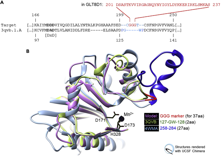    Bridging undefined template regions (step 13d)

    (A) Modification of target-template alignment for human GLT8D1 modeling on human Glycogenin-1 (PDB:3QVB). Coordinates between P126 and P129 (ends are 4.8 Å apart) are resolved in the template but extremely variable, as superposition reveals. To treat this as if the connection were undefined, G127-W128 are de-matched in addition to protocol instructions (blue font). In the resulting model the (Gly)3 bridge (red font) will align with these 2 residues in the template and replace 37 residues in the target that cannot be modeled (D201-S237, red font). It marks their insertion site. Note: (1) Alternatively, G127-W128 could be deleted from the coordinate file for 3QVB manually, and SWISS-MODEL run with this user-provided template and a target-template alignment modified exactly as per step 14d. (2) This region is known in GT-A glycosyltransferases for its conformational diversity between families (“HV2”).²⁰

    (B) 3D-Close-up showing the resulting model (lilac/red) with two template structures (blue, green). Part of the structure is removed to emphasize the conserved metal site (black stick representation, numbering is for GLT8D1).

  • f.
    For each potentially disrupting insertion or deletion noted (step 13d and step 13e), inspect and compare the sequence alignments (HHpred prediction and (sub)family MSA). Are there any potential alternative locations, i.e., alignment alternatives less disruptive for modeling but still similarly plausible at the sequence level as the original proposal? Where none can be found, use the original location predicted by HHpred.

    Note: Do not give in to the temptation to edit the target-template based on their two sequences alone, e.g., to obtain a seemingly better pair-wise percent sequence identity value. HHpred predictions have considered multiple sequence context in another way and will generally be superior to pair-wise alignment editing.

    Note:HHpred’s alignment proposals are excellent starting points and TBM is possible directly from them. Gap position readjustments are recommended out of practical consideration, to avoid unnecessary disruptive deviations from the template structure and to minimize the risk that errors could lead to loose packing and hydrogen bonding disruption within in the core regions around the active site. No general claim or evaluation is made here that gap modification by expert judgment based on 3D local structural context yields more accurate MSAs and there is to our knowledge no software that facilitates such manual intervention effectively e.g., by interactively comparing MSA scores.

  • g.
    If any gap positions remain within highly variable regions in the MSA(s), consider consolidating insertion and/or deletion sites in the target-template alignment that are near one another.

    • i.
      Verify that the 3D-location of the variable region(s) is not in the structural core.
    • ii.
      Verify that no highly conserved block in the MSA(s) is destroyed by consolidating. Otherwise, keep the multiple gaps.

      Note: Especially where score-based arbitration is precluded by the substantive evolutionary distance between the target and template proteins, consolidating gaps can help limit the number of disruptive events during TBM.

  • h.
    Make all gap shifts that you feel comfortable with in the editable target-template alignment (step 13d). If you used an [.aln] equivalent format, open the alignment in e.g., Jalview to ensure both sequences (including gaps) have the same length and that no other errors occurred while editing it manually.
  • i.
    Convert or save the aligned two sequences in FASTA format.

• 14.
  Produce 3D-structural model(s) based on user-provided target-template alignment(s).

  • a.
    Go to SWISS-MODEL’s entry page⁸ and choose “Start Modelling”.
  • b.
    Go to “Supported User Inputs” (at the time of writing located on the right side of the webpage) and choose “Target-Template Alignment”.
  • c.
    Paste or upload the alignment produced above (step 13i).
  • d.
    After automatic validation, launch by clicking on “Build Model”.

    Note: If you get an error asking to choose a Biounit, following the renaming suggestion for the template sequence and re-entering will allow you to proceed.

  • e.
    “Save all Project Data (except web files)”.

    Note: Most important among them will be the “Static Project Report”, and a file in the downloaded Archive called “model.pdb” with your model’s xyz-coordinates.

  • f.
    Examine the model visually for plausibility.

    Note: For example, inspect the model(s) in UCSF Chimera superimposed onto the template structure bundle (step 12). Be particularly attentive to any artificial poly-Gly linker that you may have introduced in step 13 to bridge regions that lacked template coordinates.

  • g.
    Renumber the structural file e.g., within UCSF Chimera (“Tools -> Structure Editing -> Renumber Residues”) so that it correctly reflects the reference numbering of your choosing (e.g., that of the UniProt entry).
  • h.
    Save your session as well as a copy in [.pdb] format (“File -> Save PDB…”).
  • i.
    Repeat steps 13-14 with any alternative template(s) and target-template alignments that you would like to consider.
  • j.
    Finally, superimpose a diverse selection of 3D-structural models (that you generated) with the bundle of template structures e.g., in UCSF Chimera like in step 12. This bundle will be helpful for designing mutations rationally in step 15.

    Note: Backbone deviation within the bundle provides a qualitative intuitive clue to the conformational diversity (and indirectly, to potentially limited accuracy) that must be anticipated in some regions. The active site region should superimpose nearly perfectly across all structures (RMSD(Calpha) <1Å).

    Note: For most human eyes, inspecting more than five homologous superimposed structures is difficult, in diverging regions even three can be challenging to follow. In most 3D-structure viewing programs, you can toggle the display of individual structures on and off while retaining them in your bundle.

    Note: Alternative excellent and reliable online TBM platforms exist. We favor SWISS-MODEL online here for two reasons primarily the option to provide a target-template alignment that is passed to the modeling process as is, and that co-crystallized entities in the template structure (including metal ions) are copied into the model if the binding residues are exactly conserved in the target. For example, our model of GLT8D1 based on XXYLT1 included the divalent cation (Mn²⁺) without further intervention due to the strongly conserved binding site in the GT-A superfamily, bound geometrically accurately in the active site.¹

    Note: There are TBM strategies also that utilize several template structures simultaneously (multiple template modeling), e.g., by averaging coordinates from automatically superimposed bundles. This may be interesting in some projects but in general, we recommend single template modeling for designing active site mutations and similar applications (where within the active site we benefit from preserving precise geometry of the potentially catalytic amino acid residues).

    Alternatives: For mutational design, we still favor manual-assisted methods but the recent successes and openness of Deep Learning developments for protein 3D-structure prediction offer a potential new shortcut to structural models in general, at least for monomeric structures. The pre-computed AlphaFold predictions are particularly promising. Based on spot-check testing their coordinates can be expected to be of very high accuracy overall, although note that they are not focused as strongly on the catalytic core domain as manual TBM protocols are i.e., any deviation from the true structure could occur anywhere in principle. Once sufficient experience has been gained in practice with using them, it is likely that protocols like ours will be revised in the future to incorporate the use of publicly available, fully automated 3D-models more generally, e.g., from the leading AlphaFold²⁵ and RoseTTAFold²⁶ efforts.

Major step 4: Design site-directed mutations to support functional investigations in the laboratory, by considering the enzymatic mechanism

Timing: ∼1 day

In GT-A glycosyltransferases, a good strategy for creating loss-of-function mutant proteins is to selectively impair the coordination of the essential divalent metal ion in its active site. The cation’s roles in catalysis may be to stabilize a nucleotide sugar donor substrate (e.g., UDP-glucose) and/or transition state conformation, and/or to engage as a Lewis acid or in another rate-enhancing interaction. Supported by a modeled 3D-structure and alignments generated as described above, we rationally designed mutants with reduced catalytic activity for GLT8D1, a member of the GT8 group of GT-A glycosyltransferases classified in Taujale et al.²⁰ This was successful despite uncertain UDP-sugar donor substrate specificity in vivo, and in absence of any knowledge regarding its acceptor substrate¹

• 15.
  Choose metal-coordinating target sites for mutation in the active site of your target.

  • a.
    In case that you used a different TBM program in step 14, or in case that SWISS-MODEL could not include a metal ion in your model because there was none reported in the template structure, you may have to infer the predicted ion position by displaying GT-A structures with coordinated metal ions in UCSF Chimera, superimposed with your model.

    CRITICAL: If the metal ion was omitted in the model, double-check that this was not due to errors in the input alignment.

    Note: For most GT-A targets, identify the residues that are primarily predicted to coordinate the Mn²⁺ (or an alternative cation) as suitable mutation sites, using the 3D-structural model.

  • b.
    For GT-A these should be three residues [DxD/H], and [H] if this motif is conserved in the target subfamily (Figure 4 in Taujale et al.²⁰).

    CRITICAL: In the (sub)family MSA from step 9 or step 10, all critical metal-coordinating residues should be conserved positions across all natural homologs if there are no errors (exceptions are very rare).

    Note: If the fourth motif is not conserved in the target MSA, focus primarily on just the two sites in [DxD/H] when designing mutations.

    Alternatives: In such cases (where the fourth motif seems to be missing) look around in the structure and MSA because an alternative, potential third metal-coordinating residue might be used in this GT-A (sub)family (and predictable). It is also possible in principle that a divergent GT-A superfamily member has lost the ability to bind a cation here. However, this would be rare and affect catalytic function (see troubleshooting problem 1).

  • c.
    Choose smaller amino acids that lack the ability to coordinate “hard” metal ions as replacement for coordinating residue(s) in the designed mutants.

    • i.
      Suitable substitution options for inhibiting the coordination of hard M²⁺ ions:

      Metal coordinating (wild-type)	Best replacement options
      Asp - D or Asn - N	Ala - A, Ser – S
      Glu - E	Ala - A, Ser - S, [Gln - Q]
      His - H	Ala - A, Ser – S

      Note: If only one of the metal-coordinating residues is mutated, we recommend alanine in order to eliminate coordination from that position. If multiple coordinating residues are mutated, structurally more similar residues could be a good alternative e.g., out of consideration for packing integrity, or to retain partial activity.

  • d.
    Based on the surrounding local 3D-structure (i.e., neighboring residues and residues from farther away in the protein sequence that are packed against the active site), could the designed mutant protein fortuitously compensate for the modification at the coordination site? All mutations should be designed with the 3D-context and geometry for the specific target protein in mind.

    • i.
      Consider whether another potential ligand residue is positioned adequately to contribute to the M²⁺ coordination sphere alternatively, specifically whether another potential ligand residue could move into the place of the original through a minor rearrangement during the folding process.
    • ii.
      If yes, then design additional custom mutation(s) to reduce this risk, if possible.

      Note: For example, in GLT8D1 and in the GT8 superfamily to which it belongs, the [DxD] motif (D171-D173 in GLT8D1 UniProt numbering) is anchored by a salt bridge between an additional aspartate residue (D172 in GLT8D1) and an arginine residue (R76 in GLT8D1). To prevent that misfolding could move this aspartate into a previously Mn²⁺-coordinating position in two prospective, single site GLT8D1 loss-of-function mutants (D171A and D173A), an additional mutation was introduced pre-emptively in each mutant (D172S). Serine was chosen here due to its similarity in size to aspartate, and its modest polarity (i.e., to neither clash nor strongly impact on folding of the arginine partner R76). The resulting mutants (mAS1:D171A+D172S and mAS2:D172S+D173A) were both demonstrably catalytically impaired.¹

      Note: It is possible in UCSF Chimera to exchange the residues in the 3D-structural model according to the designed mutations if this is desired. Except for generating illustrative images, we do not recommend doing this because accurate atomic detail here rarely required (neither for effective mutant design nor for interpreting results/observations from laboratory validation and application), and difficult to guarantee even with more advanced methods (except in rare instances when a GT-A superfamily template is used for modeling a closely related target protein).

      Alternatives: The classic rational design strategy presented here is transferable in principle to select other enzyme activities that depend on coordinating a (hard) divalent metal cation throughout their respective superfamilies, or largely throughout. At minimum, a high-level mechanistic hypothesis is required for attempts to adapt the protocol (especially to an enzyme/activity that is not related to the GT-As). This could come from specific literature about the target protein or from crystal structure or review papers about the chosen templates if they are also catalytic. Additionally, there are highly valuable online resources like EMBL’s Mechanism and Catalytic Site Atlas (M-CSA) that aim to compile the latest established information but do not contain insight for all families, yet (e.g., none was available for any GT8 family GT-A at the time of writing).

      Note: Generally, between a target enzyme and suitable templates from different (sub)families, the very central catalytic aspects and residues will often have been conserved. However, one must not expect the same for substrate specifics, or even co-factors. GLT8D1 and two viable template structure proteins within the GT8 clade,^1,20 XXYLT1 (Xyloside xylosyl transferase 1, PDB:4WMA, E.C. 2.4.2.62) and Glycogenin-1 (PDB:3QVB, E.C. 2.4.1.186) are excellent examples for this.

Major step 5: Generate site-directed mutagenesis protein overexpression constructs

Timing: ∼14 days

Timing: ∼1 week (for step 16)

Timing: ∼1 h (for step 17)

Timing: ∼1 week (for step 18)

In this part of our protocol, we describe the generation of several protein expression constructs to verify the in silico predicted enzymatic activity, as well as to reveal whether the designed substitutions of in silico predicted active site residues (step 15b and step 15c) affect the enzymatic activity of the protein under investigation (Figure 4). Specifically, we describe the actual experimental set-up for generating the GLT8D1 mutation constructs used for the study Ilina et al.,¹ but this protocol can be adapted to generate different overexpression constructs.

CRITICAL: Ensure that your target vector contains the right elements to ensure proper and high expression in the cell system used for recombinant protein expression in major part 6 of this protocol. Important regulatory elements of our vector system used, resulting in high protein yield when executing following overexpression protocol are schematically illustrated in Figure 5. Comparable overexpression constructs can be used (for more information read Makrides²⁷).

Note: Vector-specific properties (e.g., position of restriction sites) have to be considered before starting this protocol section and adjusted respectively if required.

• 16.
  Generate overexpression construct of wild-type target protein.

  Note: The commercially available vector carrying the gene of our interest (GLT8D1) already contained a C-terminal HA-tag (pcDNA3.1-GLT8D1-HA).

  Alternatives: We used the hemagglutinin-tag (HA-tag) containing vector, as this is a standard in our laboratory. Alternatively, one may use other vectors with different tags, also with different tag localization (N- or C-terminal), depending on the protein of investigation. If there’s no commercial tag-carrying vector available, one can design and add an extra step to clone the gene sequence of interest in the pcDNA3.1-”Tag-of-interest” vector.

  Note: This protocol describes the cloning strategy of the tagged gene sequence from the commercially available vector into another vector suitable for lentiviral particle production (pCDH-EF1α-IRES-Neo) since the next steps of our experimental set up in Ilina et al.¹ included transduction of cells with DNA sequence of the construct under investigation. However, a lentiviral plasmid backbone is not necessarily required for this protocol.

  • a.
    Amplify the tagged insert (GLT8D1-HA) using primers that introduce XbaI and NotI restriction sites to generate XbaI-GLT8D1-HA-NotI insert.

    • i.
      Prepare the PCR reaction mix as follows using primer set #1 (see key resources table):
      PCR reaction mix

      Reagent	Amount
      DNA template (pcDNA3.1-GLT8D1-HA vector)	X μL (calculate for 100 ng)
      DNA polymerase (Phusion Hot Start Polymerase)	0.5 μL
      Primer set (10 μM)	1 μL
      5× HF buffer (or GC buffer)	10 μL
      10 mM dNTP	1 μL
      ddH20	Up to 50 μL

      Note: Prepare primer mix in advance (1:1 mix of forward and reverse primers, final concentration 10 μM).

      Note: Master mix of water, buffer, dNTPs and polymerase can be prepared for several reactions if amplification of different template DNAs with different primers is planned in parallel.

      Alternatives: We used Phusion Hot Start polymerase from ThermoFisher Scientific that is less sensitive to the temperatures on ice. Alternative products can be used e.g., from NEB (#M0530) or APExBIO (#K1031) but the protocols need to be adapted according to manufactures recommendations.

    • ii.
      Run PCR under following conditions using an annealing temperature of 61°C:
      PCR cycling conditions

      Steps	Temperature	Time	Cycle(s)
      Initial Denaturation	98°C	30 s	1
      Denaturation	98°C	10 s	30
      Annealing	XX°C	30 s
      Extension	72°C	30 s
      Final extension	72°C	10 min	1
      Hold	4°C	Forever

      Alternatives: Annealing temperature highly depends on the primers used. Please verify it for your primers and adjust the PCR program, if necessary.

      Pause point: Rest on ice (up to 1 h) or store at -20°C until proceeding to the next step.

  • b.
    Purify the insert (GLT8D1-HA) via gel electrophoresis on agarose.

    • i.
      Prepare 1% agarose gel with Ethidium Bromide.

      Alternatives: if your lab is Ethidium Bromide-free, GelRed^TM or GelGreen^TM can be used as an alternative.

    • ii.
      Load 50 μL of the PCR product mixed with 8 μL of 6× Gel Loading Dye and run for 60 min at 120 V.
    • iii.
      Check the band size with the UV light, excise the correct sized band (for GLT8D1 amplicon with restriction sites: 1,177 bp).

      CRITICAL: do not to expose the gel to the UV light for too long, since it may lead to undesired DNA damage.

    • iv.
      Perform the gel elution with QiaQuick gel extraction kit according to the manufacturer's protocol.

      Alternatives: Other DNA gel elution kits can be used e.g., GeneJET Gel Extraction Kit, Monarch® DNA Gel Extraction Kit or Zymoclean Gel DNA Recovery Kits.

    • v.
      Measure the concentration of the eluted DNA using a photometer (e.g., Nanodrop or similar device).

      Pause point: Rest on ice (up to 1 h) or store at −20°C until proceeding to the next step.

  • c.
    Perform restriction digest of empty vector (pCDH-EF1α-IRES-Neo) and the (insert GLT8D1-HA) with XbaI and NotI enzymes.

    • i.
      Prepare the digestion mix for each digestion probe as follows:

      Reagent	Amount
      DNA	1 μg
      10× NEB CutSmart Buffer	5 μL
      XbaI	1 μL
      NotI-HF	1 μL
      Nuclease-free H20	Up to 50 μL

      Alternatives: If your protocol requires different restriction enzymes, make sure to adjust the restriction buffer, respectively.

      Alternatives: restriction enzymes from other companies than New England Biolabs, e.g., Thermo Scientific Restriction & Modifying Enzymes.

    • ii.
      Gently mix the reaction by pipetting up and down and microfuge briefly.
    • iii.
      Incubate at 37°C for 2 h.
    • iv.
      For de-phosphorylation of the backbone add 2 μL of Alkaline Phosphatase in the vector digestion mix.
    • v.
      Incubate at 37°C for 30 min.
    • vi.
      Inactivate restriction enzymes at 65°C for 20 min.

      Pause point: Rest on ice (up to 1 h) until proceeding with the next step. Alternatively, store at −20°C.

  • d.
    Purify insert (GLT8D1-HA) and open vector (pCDH-EF1α-IRES-Neo) via gel electrophoresis on agarose (according to step 16b). Excise GLT8D1 insert of 1,177 bp and pCDH-EF1α-IRES-Neo vector fragment of 7,845 bp.
  • e.
    Ligation of purified vector (pCDH-EF1α-IRES-Neo) and insert (GLT8D1-HA).

    • i.
      Prepare vector-insert (1:3) and vector only (negative control) mixes for ligation procedure as follows:

      Reagent	Amount
      Quick Ligase Reaction Buffer (2×)	5μL
      Vector DNA (7.8 kB)	0.020 pmol
      Insert DNA (1.1 kB)	0.060 pmol
      Quick Ligase	0.5 μL
      Nuclease-free H20	Up to 10 μL

      Note: Vector-to-insert ratio is defined by their molar mass. Biomath Calculator is a useful online tool for calculation.

      Alternatives: Other ligases alternatively to NEB Quick ligase can be used e.g., T4 DNA Ligase from ThermoFisher or T4 DNA Ligase from Promega. The protocol needs to be adapted accordingly to the respective manufacturer's recommendations.

    • ii.
      Gently mix the reaction by pipetting up and down and microfuge briefly.
    • iii.
      Incubate at 20°C–25°C for 5 min.
    • iv.
      Rest on ice until (up to 1 h) proceeding to the next step.
  • f.
    Plasmid amplification and purification (pCDH-EF1α-GLT8D1-HA-IRES-Neo).

    • i.
      Prepare the LB agar plates with Carbomycin antibiotic (100 μg/mL).
    • ii.
      Transform 1 μL of the reaction into 50 μL of competent cells (NEB Stbl. E.coli) and incubate for 30 min on ice.

      Alternatives: Depending on the bacterial strain used, the type of media and/or antibiotics may vary. Please verify it with your available laboratory materials/equipment before starting.

    • iii.
      Heat shock for 35 s at 42°C and place on ice afterwards.
    • iv.
      Add 400 μL of low salt LB media into the bacteria and pipette up and down gently.
    • v.
      Transfer the bacteria on agar plates: one plate for ligation product of vector and insert and one plate for ligation product of vector only (as a negative control). Turn the plates upside down and incubate 16–20 h at 37°C.

      CRITICAL: Upside-down placement is necessary to prevent formation of water condensate onto the agar that would prevent formation of single bacterial colonies.

    • vi.
      Check the plates for ratio (ligation vs. control) and decide if 1–3 colonies can be expanded.

      CRITICAL: If there is no difference in the colony numbers between the control and the ligation plates, the ligation reaction most likely did not work. Repeat the ligation reaction (including new negative control) again before proceeding with the next step.

    • vii.
      Expand 1–3 colonies by picking the single colonies and transferring them to the LB medium (5 mL).
    • viii.
      Incubate the picked colonies at 37°C 16–20 h, while shaking (220 rpm).

      Alternatives: in the current set-up we used colony expansion followed up with plasmid isolation and quality control, as the colony yield and quality check revealed good results. Alternatively, an additional step of colony PCR on a larger number of colonies (e.g., 8–16) can be introduced prior to plasmid isolation.

    • ix.
      Perform plasmid preparation for each colony with Macherey-Nagel Nucleospin plasmid kit according to manufacturer’s protocol.

      Alternatives: Other commercial available kits for plasmid preparation can be used instead e.g., ZymoPURE Plasmid Miniprep Kit, Monarch® Plasmid Miniprep Kit or QIAprep Spin Miniprep Kit.

    • x.
      Measure the concentration of the plasmid DNA using a photometer (Nanodrop or similar device).
    • xi.
      Send the plasmids for Sanger sequencing using primers located within the backbone. Proceed only with plasmids with mutation-free sequencing results.

      Pause point: Store plasmid DNA at −20°C until further use.

• 17.
  Design PCR primers for overlapping PCR to introduce desired mutations in your target proteins DNA sequence.

  • a.
    Design primers manually or by using appropriate software e.g., we recommend designing overlapping PCR primers by using a SnapGene software according to a standard manufacturer’s protocol. The tool “modify the primer” can be used to introduce a point mutation in the desired sequence.

    Alternatives: we used SnapGene software for visualization of cloning strategy and primer design since it is the standard software used in our laboratory; however, different software or programs may be used for any of this, depending on laboratory preferences and licenses (e.g., free software ApE plasmid editor or Benchling).

  • b.
    Order the oligo sequences at your company of choice using standard synthesis parameters (e.g., 10 nmol, 100 μM, without additional modifications, SePOP purified).
• 18.Generate mutation constructs by overlapping PCR.
  This step aims to generate a eukaryotic overexpression vector (pCDH-EF1α-IRES-Neo) that carries tagged insert (human GLT8D1-HA) with mutations in the metal ion-coordinating amino acids predicted to be crucial for its enzymatic activity (in step 15b).

  Note: This section describes the constructs we generated during our study.¹ The first construct, named mAS1, generates a mutant protein in which asparagine (D) on position 171 is replaced by an alanine (A) and D172 is replaced by a serine (S) (pCDH-EF1α- GLT8D1[D171A/D172S]-HA-IRES-Neo). The second construct, named mAS2, generates a mutant protein in which D171 is replaced by an S and D173 by an A (pCDH-EF1α-GLT8D1[D172S/D173A]-HA-IRES-Neo).

  • a.
    Generate two overlapping fragments of the insert (GLT8D1-HA) carrying point mutations by PCR amplification of the wild-type sequence generated in step 16 (pCDH-EF1α-GLT8D1-HA -IRES-Neo). Use the custom-designed primers from step 17 (see key resources table; Primer set #2 + #3 for mutation mAS1; Primer set #4 + #5 for mutation mAS2).

    • i.
      Repeat step 16a and step 16b to amplify and purify overlapping, mutated insert fragments 1 and 2. Excise the insert fragments of 548 bp (fragment 1) and 663 bp (fragment 2).
  • b.
    Perform an overlapping PCR to generate mutated insert sequence carrying mAS1 or mAS2 point mutations (mAS1: XbaI-GLT8D1(171ASD173)-HA-NotI, overlapping region between the fragments: 34 bp; mAS2: XbaI-GLT8D1(171DSA173)-HA-NotI, overlapping region between the fragments: 35 bp). The PCR program is carried out in two consecutive steps:

    • i.
      The PCR mix containing both fragments, buffer, dNTPs, polymerase and water undergoes several PCR cycles to make sure that full length insert is produced from the two annealing fragments.
      PCR reaction mix

      Reagent	Amount
      DNA template (fragment 1 + fragment 2 in a proportion 1:1)	X μL (calculate for 100 ng)
      DNA polymerase (Phusion Hot Start Polymerase)	0.5 μL
      5× HF buffer (or GC buffer)	10 μL
      10 mM dNTP	1 μL
      ddH20	Up to 50 μL

      Alternatives: We used Phusion Hot Start polymerase from ThermoFisher Scientific that is less sensitive to the temperatures on ice. Alternative products can be used e.g., from NEB (#M0530) or APExBIO (#K1031) but the protocols needs to be adapted according to manufacturer's recommendations.

    • ii.
      Run 11 cycles of PCR.
      PCR cycling conditions

      Steps	Temperature	Time	Cycles
      Initial Denaturation	98°C	30 s	1
      Denaturation	98°C	10 s	11 cycles
      Annealing	55°C	20 s
      Extension	72°C	1 min
      At this step pause the cycler and add the primers mix as described in the next steps.

      CRITICAL: This step allows amplifying the full-length sequence carrying desired mutations, but the quantity of PCR product will not be enough for cloning. Therefore, it is crucial to proceed with the next steps (adding primers and running the second step of the PCR).

      Alternatives: Annealing temperature highly depends on the primers used. Please verify it for your primers and adjust the PCR program, if necessary.

    • iii.
      Add 1 μL of the primer set #1 (see key resources table) to each reaction tube and run additional 25 cycles of PCR under following conditions to amplify the full length sequence that carries the desired mutation and restriction sites.

      Note: One primer mix is used for amplification of both mutants, since these primers are located outside of the mutated regions and are for the full-length sequence.

      PCR cycling conditions

      Steps	Temperature	Time	Cycle(s)
      Initial Denaturation	98°C	30 s	1
      Denaturation	98°C	10 s	25
      Annealing	60°C	20 s
      Extension	72°C	1 min
      Final extension	72°C	5 min	1
      Hold	4°C	forever

      Alternatives: Annealing temperature highly depends on the primers used. Please verify it for your primers and adjust the PCR program, if necessary.

      Pause point: Rest on ice until proceeding with the next step (up to 1 h). Alternatively, store at −20°C.

  • c.
    Repeat step 16b. Excise the mutation-carrying mutant inserts (GLT8D1-HA inserts of 1,177 bp).
  • d.
    Restriction of empty vector (pCDH-EF1α-IRES-Neo) and the inserts (GLT8D1-HA) carrying mAS1 or mAS2 point mutations with XbaI and NotI enzymes according to step 16c.
  • e.
    Repeat step 16b to purify the insert (mAS1-GLT8D1-HA or mAS2-GLT8D1-HA) and the open vector (pCDH-EF1α-IRES-Neo). Excise mutation-carrying insert (GLT8D1-HA of 1,177 bp) and vector fragment (pCDH-EF1α-IRES-Neo of 7,845 bp).
  • f.
    Ligate the purified mutation-carrying inserts (mAS1-GLT8D1-HA or mAS2-GLT8D1-HA) and the vector (pCDH-EF1 α -IRES-Neo) according to step 16e, following plasmid expansion and preparation following the steps noted in step 16d.

    Alternatives: in the current set up we used the overlapping PCR method for introducing point mutations in the plasmid, as it is a standard established technique in our laboratory. Alternatively, commercially available mutagenesis kits (e.g., QuikChange® Site-Directed Mutagenesis Kit or Q5® Site-Directed Mutagenesis Kit) may be used, especially if they are already established as a standard technique in your laboratory.

Figure 4.

Schematic illustration of experiments described in major step 5 (steps 16–18)

Figure 5.

Regulatory elements included in our expression plasmid useful for an increased protein expression

The human elongation factor promotor (EF1α) is known to drive high and efficient gene expression²⁸; the woodchuck hepatitis virus posttranscriptional regulatory element (WPRE) is a DNA sequence that upon transcription creates a tertiary structure enhancing insert expression; the SV40 poly-A sequence promotes transcript stability; the origin of replication (ORI) from SV40 enables the construct to be replicated in cells that express the SV40 large T antigen such as 293T cells that are used within described protocol.

Major step 6: In vitro glycosyltransferase activity assay

Timing: ∼3 days

Timing: ∼4 h (for step 19)

Timing: ∼1 h (for step 20)

Timing: ∼3 h (for step 21)

Timing: ∼1 h (for step 22)

Timing: ∼3 h (for step 23)

An in vitro assay should reveal whether the substitution of the in silico predicted active site amino acids affects the enzymatic activity of the protein under investigation. For this purpose, wild-type and mutated versions (wt, mAS1, mAS2) of the protein of interest will be overexpressed, purified and used for an in vitro glycosyltransferase activity assay (Figure 6). The following section describes the use of Hek293T cells as mammalian cell-based recombinant protein expression system.

Alternatives: Cell-free protein synthesis or other host systems for recombinant protein expression can be used e.g., from insect, yeast, bacterial or algal depending on the origin and properties of the protein under investigation.^29,30 In general, one should use a cell system matching to the origin of the protein under investigation.

• 19.
  Transfect Hek293T cells using CaCl₂-BES transfection method.

  Note: Mutated proteins will be overexpressed in Hek293T cell by transiently transfecting the cells with the respective plasmid DNA. There are several protocols for how to transfect cells. We used the CaCl₂-BES transfection method as it is low cost. Calcium phosphate forms an insoluble precipitate with DNA, this complex then attaches to the cell surface where it is transported into cells by endocytosis. However, lipofection yields a higher transfection efficiency resulting in increased recombinant protein expression and should be preferably used over CaCl₂-BES transfection when noticing insufficient protein amounts after immunoprecipitation (IP).

  Alternatives: We used the Hek293T human embryonic kidney cell line to overexpress our protein of interest. Hek293T cells express the SV40 large T antigen and therefore produce high amounts of recombinant proteins when using overexpression plasmids containing SV40 ORI. However, other mammalian cell lines can be used as well e.g., HeLa cells. For a review about general considerations to make when planning recombinant protein overexpression in mammalian cells, please refer to Khan.³¹

  • a.
    Seed 3 × 10⁶ Hek293T cells in a 10 cm dish (around 30% confluence) in 10 mL culture media. Incubate the cells for at least 3 h at 37°C, 5% CO₂ in a humidified atmosphere.
  • b.
    Dilute 25 μg of plasmid DNA in 375 μL ddH₂O. Add 125 μL of 1 M CaCl₂ and mix by pipetting up- and down several times. Slowly add 500 μL 2×BES solution dropwise into the DNA-CaCl₂ mixture and incubate for 20 min at room temperature.

    Note: The formation of calcium phosphate DNA complexes becomes visible in the formation of fine haze.

    CRITICAL: As the pH of the 2×BES solution is critical for proper complex formation, all solutions need to be adjusted to room temperature before use.

    CRITICAL: It is very important to carefully and drop-wise add the 2×BES solution to the DNA-CaCl₂ mix.

    CRITICAL: Do not extend incubation time, as this will lead to increased aggregation of particles.

  • c.
    After incubation apply the mix drop-wise onto the Hek293T cells and place the cells back into the incubator.

    Note: Particles should appear as fine haze under the microscope.

    Note: Cell number and reagents can be scaled up and down if required. We would recommend to maximum prepare a transfection-mix of 1 mL volume total, meaning that if you plan to upscale the experiment don’t upscale the reaction mix; instead prepare several mixes of max. 1 mL total. Increasing the volume leads to reduced formation of CaCl₂-BES-DNA crystals.

• 20.
  Harvest transfected cells and perform target protein extraction.

  • a.
    Re-fresh the media after 6–10 h post transfection.

    CRITICAL: Longer incubation times will increase cell death.

  • b.
    Collect the cells 48 h post transfection,

    • i.
      Flush them two times with ice-cold PBS.
    • ii.
      Add 2 mL of ice-cold PBS, and directly scrape the cells off the surface.
    • iii.
      Quickly collect the cells in a 15 mL tube on ice.

      Note: Scraping already destroys the outer membrane and thereby increases lysis efficiency. One can use trypsin instead to detach the cells from the surface but be careful as trypsin might interfere with your protein of interest.³²

  • c.
    Centrifuge the cells for 3 min at 300 g and remove the supernatant.

    Note: No pause point at this step, directly proceed to protein extraction as freeze thawing seems to affect enzyme activity and might change results of the activity assay.

    Note: All steps of protein extraction should be strictly performed on ice or at 4°C.

  • d.
    Lyse the cell pellets in non-denaturing extraction buffer for 30 min on ice, while pipetting up and down several times each 10 min of incubation.

    Alternatives: Adapt your extraction buffer if required depending on the properties of your protein of interest.

    CRITICAL: The detergent used in this buffer is relatively gentle and allows solubilization of proteins that retain enzymatic activity, but this may result in extractions that are less complete than with extraction buffers using detergents that are more stringent. Eventually upscale amount of cells to compensate for that effect.

    Note: The amount of lysis buffer applied is dependent on the size of the cell pellet. As a rule of thumb, the volume of protein extraction buffer should be three times the volume of cell pellet. We usually applied 500 μL protein extraction buffer on a cell pellet collected from an 80%–90% confluent 10 cm plate of Hek293T cells.

  • e.
    After lysis, centrifuge for 15 min 16.000 g at 4°C, transfer the supernatant in a fresh tube and discard the pellet.

    Note: No pause point. Directly proceed to immunoprecipitation.

• 21.
  Purify target protein by immunoprecipitation.

  Note: All steps of IP will be strictly performed on ice or at 4°C and with ice-cold buffers and solutions.

  • a.
    Wash 50 μL Anti-HA Magnetic Beads per IP reaction 3 times in each 300 μL extraction buffer.

    • i.
      Completely remove liquid after the last wash.
    • ii.
      Use a magnetic bar to separate magnetic beads from supernatant efficiently.

      Alternatives: When using a different tag than HA on your protein of interest use other coupled beads. We strongly recommend using a tagged protein for this experiments as this allows for peptide elution increasing the yield. Native elution without peptide is possible but requires adaption.

  • b.
    Apply the 500 μL protein extract onto the HA-magnetic beads and incubate for 1 h rotating at 4°C.

    Note: Seal the tubes containing the cell lysate-bead mix (e.g., with parafilm) to prevent leakage.

  • c.
    Separate the protein-coupled magnetic beads from the supernatant using a magnet.
  • d.
    Wash the protein-coupled magnetic beads twice with each time 300 μL lysis buffer.
  • e.
    Wash one time with 300 μL PBS.

    • i.
      During each washing step, invert the tube several times delicately.
  • f.
    Remove liquid completely after the last washing step and re-suspend the protein-coupled beads in 50 μL HA synthetic peptide solution (c: 1 μg/μL in PBS) for target protein elution.
  • g.
    Incubate for 1 h rotating at 4°C.
  • h.
    Separate beads from supernatant containing the protein.
  • i.
    Transfer the supernatant into a fresh tube and discard the beads.

    Optional: Before proceeding with IP, keep a small fraction of the cell extract as an input control for immunoblot (about 1/20). Collect once more a 1/20 supernatant as control for immune blot. To validate efficiency of immunoprecipitation, control samples for input and supernatant were analyzed by immunoblotting. Ideally, the amount of detectable target protein by incubation with an antibody against the HA-tag reduces dramatically after immunoprecipitation.

    Note: No pause point. Directly proceed to the next step.

• 22.
  Determine protein concentration of purified protein.

  Alternatives: We used the Pierce BCA protein assay suitable for the detection of protein concentrations as low as 5 ng/μL. If you expect lower amounts or face problems detecting proteins using this kit, you can use other assays that are suitable for protein concentrations as low as 0.5 ng/μL (e.g., the BCA protein assay kit for low concentrations from abcam #ab207002).

  • a.
    Dilute 2 μL of your elution sample in 48 μL PBS to prepare a 1:25 dilution.
  • b.
    Pipette 25 μL of your sample-dilution in duplicates into a well of a U-bottom 96 well plate.
  • c.
    Apply 25 μL of each standard in duplicates onto the plate. The standard is composed of the following BSA concentrations in PBS: 0 ng/μL, 5 ng/μL, 25 ng/μL, 50 ng/μL, 125 ng/μL, 250 ng/μL.
  • d.
    Add 25 μL of the working reagent prepared according to the instruction of the manufacturer into each well and mix using a plate shaker for 30 s.
  • e.
    Seal the plate using parafilm or sealing tape and incubate for 30 min at 65°C.
  • f.
    After incubation, quickly centrifuge the plate for 1 min at 300 g and cool the plate down to room temperature. Remove the tape and measure the absorbance at 562 nm using a plate reader.
  • g.
    Determine the protein concentration of your sample.

    • i.
      Calculate the average of each duplicate (sample and standard).
    • ii.
      Subtract the value of the blank standard (0 ng/μL) from all other values.
    • iii.
      Prepare a standard curve by plotting the average blank–corrected 562 nm measurement value for each BSA standard according to its concentration in ng/μL.
    • iv.
      Use the standard curve to determine the protein concentration of your sample.

      Note: On average we yield concentrations around 30–50 ng/μL for each IP we performed according to this protocol.

• 24.Determine enzymatic activity of target protein by glycosyltransferase assay.
  We used the Promega UDP-Glo™ glycosyltransferase bioluminescent assay to detect glycosyltransferase activity of our target protein. Following the glycosyltransferase reaction, free UDP is converted into ATP, which is then converted into a luminescent signal that is proportional to the glycosyltransferase activity in the reaction. We designed our glycosyltransferase assay to analyze GLT8D1 wild-type and mutant (mAS1, mAS2) enzyme velocity for two different glycosyltransferase donor substrates (UDP-glucose and UDP-galactose).

  Alternatives: Based on the in silico sequence analysis we expected that our protein of interest possesses glycosyltransferase activity. More specifically, we were able to propose already a donor substrate preference for a hexose, possibly glucose. If your protein of unknown function shows similarities to enzymatic protein families other than the GT-A glycosyltransferases, you should use an activity assay designed to detect the respective enzymatic activity.

  Note: We used the UDP-Glo^TM Glycosyltransferase Assay kit from Promega and slightly adapted the manufacturer’s instructions. To determine kinetic parameters of the glycosyltransferase reaction, multiple reactions with varying concentrations of the respective substrate were carried out simultaneously.

  Note: We took advantage of the fact that HA peptide can be an acceptor substrate for N-linked glycosylation.³³ For this reason, we did not apply any additional acceptor substrate in our reaction.

  Note: We performed several glycosyltransferase activity assays in advance to figure out the optimal volumes, concentrations and conditions.

  Note: Ideally, the reactions are performed at least in duplicates.

  • a.
    Prepare each set of reactions in a 384 well plate as follows:

    Ingredient
    Donor substrate	0 μM	100 μM	1,000 μM	5,000 μM	10,000 μM
    Purified peptide	100 ng	100 ng	100 ng	100 ng	100 ng
    Glycosyltransferase reaction buffer	1 ×	1 ×	1 ×	1 ×	1 ×

    Note: in addition to the peptides under investigation, we applied one set of reactions without peptide as no-peptide control.

  • b.
    Prepare a UDP-standard with the following concentrations in glycosyltransferase reaction buffer: 0 μM, 0.1 μM, 1.56 μM, 6.25 μM, 25 μM. Apply 10 μL of each standard concentration on the 384 well plate.
  • c.
    Incubate the plate for 1 h at 37°C.
  • d.
    After incubation, add 10 μL of detection reagent prepared according to the manufacturer's instructions to each well and mix 30 s using a plate shaker.

    Note: This step terminates the reaction.

  • e.
    Incubate the plate for 1 h at room temperature protected from light.
  • f.
    Transfer each sample into a well of a white flat bottom 96 well plate.
  • g.
    Measure the luminescence signal (endpoint) using a plate reader. See Figure 7 for an exemplary plate set-up.
  • h.
    Refer to Figure 8 and the quantification and statistical analysis section of this protocol for our method of glycosyltransferase activity assay data analysis.

Figure 6.

Schematic illustration of experiments described in major step 6 (steps 19–23)

Figure 7.

Exemplary set-up of a 96-well plate for luminescence measurement after glycosyltransferase activity assay (step 23)

The reaction of each peptide with respective substrate concentration is applied in duplicates. Reactions incubated without peptide but with varying substrate concentrations serve as no-peptide control required for later quantification. UDP-standard ranging from 0 μM–25 μM is also applied in duplicates onto the plate.

Figure 8.

Workflow—Determination of the substrate turnover rate based on the results of the glycosyltransferase assay (step 23)

Expected outcomes

This protocol consists of three major parts: rational 3D-model-based design of protein active site mutations (major steps 1–4), cloning of protein coding sequence into an eukaryotic overexpression vector and introduction of point mutations resulting in substitution of amino acid residues crucial for active site function (major step 5), and validation of the decreased enzymatic activity by functional assay (major step 6). We have successfully demonstrated that this workflow can be used to predict and validate the amino acid residues accounting for enzymatic activity of the formerly unknown protein GLT8D1.¹

The expected outcomes for the first part of our described protocol are (i) high-quality target (sub)family MSA and 3D-structure model(s) that can be used to support/generate your research hypothesis beyond the active site prediction, and (ii) the in silico generation of mutant sequences of likely catalytically impaired variants of the target protein. The main expectation for the cloning part is generation of undesired-mutation-free and desired-mutation-only-containing protein.

During each bacterial transformation step (colony formation), we observed a significantly higher number of colonies on the construct-containing plate and negative control (vector-only) plate. Ideally, the negative control plate contains no or very few colonies, while the construct-carrying one has a substantive amount of colonies to choose from. The ratio of colonies on construct-containing plate vs. control-plate is crucial when deciding the number of colonies to be propagated for a quality control by Sanger sequencing. If both plates show comparable amounts of colonies, the experiment did not work well and the entire step should be repeated.

The last part of this protocol intends to determine the consequence of site-directed mutations of in silico predicted active site residues for the enzymatic activity of the protein under investigation. After Hek293T cell transfection, protein extraction and immunoprecipitation following described parameters we yield on average concentrations around 30–50 ng/μL for each IP. Our glycosyltransferase activity assay performed under described conditions resulted in a stable and reproducible increase in turnover rate with increasing substrate concentration. In addition, all values we obtained were clearly increased in comparison to the “no-peptide” control values.

Quantification and statistical analysis

Determination of the substrate turnover rate based on the results of the glycosyltransferase assay step 23 (Figure 8).

During the glycosyltransferase activity assay, the released UDP product is converted to adenosine triphosphate (ATP) that generates light in a luciferase reaction. The relative light unit (RLU) values generated correlate to the free UDP concentration and can be determined by using a UDP-standard curve. For detailed information about the UDP-Glo™ Glycosyltransferase Assay, read the manual provided by Promega. We have used this protocol to describe the substrate turnover rate (μM/h or nmol/s) for our wt peptide and compared it to the substrate turnover rates of our two active site mutation peptides to draw conclusions if enzymatic activity under the applied conditions is impaired.

Alternatives: The results of the glycosyltransferase assay could be in principle used to determine enzyme kinetic parameters V₀, V_max and K_m if the data fit the criteria required. However, we do not describe this calculation in detail but recommend to follow the GraphPad Prism tutorial or to follow the protocols described in McGraphery and Schwab³⁴ or Augustin and Bak³⁵ if aiming to determine potential enzyme kinetics.

• 1.Subtraction of background RLU values.

After successful execution of all protocol steps, you will have a tabular (e.g., in Excel) file containing the RLU values after 1 h glycosyltransferase reaction for each of your wells filled with sample. If you have applied, your samples in duplicates (which is recommended) first calculate the mean value for each sample. Subtract the RLU value of the 0 μM samples (UDP-standard and UDP-substrate) from the other values of respective condition. Subtract as well the RLU value of the no-peptide control of given substrate concentration from the other values of respective condition. The results are the RLU background corrected values of your measurement.

• 2.Generation of the UDP-standard curve.

To correlate the RLU values you have received for each reaction with the amount of free UDP you have to generate the UDP-standard curve by using your values. Plot the concentration values of the UDP-standard against the respective RLU values and determine the linear regression line and equation using e.g., Excel.

• 3.
  Using the line equation of UDP-standard curve to express your results in nmol UDP per second (nmol/s).

  • Solve the line equation for x and apply on your sample RLU values to calculate the substrate turnover rate in μM/h for each condition. Divide each value by 3.6 to express the substrate turnover rate in nmol/s.
• 4.Graphical representation of your results.

The results can be represented as bar graphs or in a scatter plot, plotting applied substrate concentration against the substrate turnover rate calculated in step 3. Scatter plot with non-linear regression line is the most common way reaction rates of enzymes are displayed and can be used to determine enzyme kinetic parameters.

Optional: When aiming to determine kinetic parameters of your protein under investigation we recommend using the GraphPad Prism software. Additional instructions for the calculation and how to use Graphpad Prism for that purpose can be found here.

Limitations

Each enzyme family is different and dissecting the detailed mechanistic steps and roles for individual members of each residue necessitates a long interplay of theoretical hypotheses and designed experiments for ultimate verification. Whether that is required for designing mutations depends on the enzyme family and on the project constraints and goals. Generally, designing loss-of-function mutants will be feasible, e.g., via this protocol. A trained protein biochemist armed with a 3D-structure that accurately reflects the active site geometry and proximal residues (even if modeled) and high-quality MSAs will be able to rationally design powerfully and selectively inhibiting point mutations in any target enzyme (i.e., where otherwise the integrity of folding, structure, and unassociated molecular functions are unaffected). This is done by relying on current knowledge, from educational resources in print and online, to infer frequently observed mechanistic roles and chemical patterns in enzymes (e.g., general acid-base catalysis, involvement of metal ions in catalysis, etc.), and on knowledge of which amino acid side-chains are chemically capable to assume such roles. While not all active site residues are absolutely conserved and not all conserved residues are catalytically crucial, it is easy to recognize candidate players (and candidate mutation sites) in MSAs, especially if enzyme activity has been conserved throughout the family. Conversely, designing gain of function mutants is much more difficult and successful primarily in cases where natural inhibitory interactions can be removed through mutation.

During in vitro generation and testing of the loss-of-function mutants, each protocol step bears some risk of producing artifacts, especially if not enough accuracy and attention to conditions and details is given. Following all advices marked as “CRITICAL” in this protocol should help to control these risks. The quality of materials used must be good (no repeated thaw-freeze cycles for sensitive ingredients of bacterial strains) and the temperature and buffer conditions should be optimal. Some experimental conditions we applied in our experiments should be adapted if required. For example, too stringent or too soft temperature conditions at the annealing stage (especially at the step of overlap PCR) may result in failure for primers to anneal or in unspecific primer binding and sabotage your PCR product.³⁶

Another, general limitation of assaying enzyme activity in vitro is that the protein of interest is transiently overexpressed at non-physiological levels, which may prevent accurate protein folding, prevent or induce posttranslational modifications or lead to proteolytic cleavage. This could affect the activity determined by the enzymatic assay to a degree. Additionally, introducing a small HA peptide tag to facilitate immunoprecipitation and native elution could interfere with protein structure and function. Note however that both techniques are widely used successfully in protein engineering (as well as protein expression for structure determination) and with a 3D-model in hand already linkers can be conceived that minimize this risk. It is worth remembering here that any catalytic activity that is measured for a mutant or wild-type protein verifies native-like folding at least of a proportion of expressed protein through viability of its active site geometry, and rules out a categorical refolding problem. It is therefore not necessary in practice to undertake the effort (time and cost) to determine the structure of every mutant experimentally. Ultimately, if one of the tools proves particularly useful in further research through its mutation, and if high-resolution detail is of interest, “proof” through e.g., a crystal structure is of course always desirable.

Although transient overexpression in Hek293T cells is widely used, alternative transfection approaches including lipofection and lenti- or adenovirus mediated gene delivery may be considered in other cell types. Using the right assay to determine the enzymatic activity of purified protein is crucial. Finally, the enzymatic assay chosen, and its parameters, should match the target protein’s physiological function as best as possible. If unknown, predictions or hypotheses based on literature research will be helpful initially to guide reaction buffer composition, donor and acceptor substrates, like it was for GLT8D1.¹ Ultimately, screening approaches and potentially the mutants designed and validated on these hypotheses can be utilized to elucidate the physiological substrate(s), and thereby enable more meaningful kinetic studies. Even though described protocol could be successfully used to achieve impaired enzymatic activity of a GLT8D1 mutation construct, we were not able to determine the enzymatic kinetics parameters. Possible explanations are that we did not use the physiological substrate in our in vitro assay or that the substrate concentration for saturation of enzymatic reaction was not reached.

Troubleshooting

Problem 1

Positions that are known to be very highly conserved and important for catalysis are not fully conserved in the target (sub)family MSA and this is neither due to erroneous sequences nor to misalignment as far as this can be established (step 1d).

Potential solution

The target protein may not be catalytic (even if related protein families are). Therefore, before engaging in time-intensive analyses and mutant production, consider verifying that enzymatic activity can be demonstrated in vitro for the wild-type target protein.

Note: Inferred functional annotation for a superfamily (e.g., E.C. codes in Pfam or even in UniProt records) can be misleading. It does not imply that all members of the superfamily or family have retained this property necessarily.

Problem 2

Few error-free homolog sequences are available and this prevents that a rich and diverse MSA of the target (sub)family can be generated using OrthoMCL (steps 2-9).

Potential solution

First, try alternative ortholog resources, e.g., OMA. If unsuccessful then assembling, an MSA by BLAST searches against other databases beside UniProt may yield a (sub)family MSA that at least over the fragment of interest is relatively low in errors, if carefully pruned. Alternatively for GT-A targets, consider using the sequences clustered with the target protein by Taujale et al.²⁰ If neither approach yields a persuasively correct set of aligned sequences nor this issue cannot be remedied then proceed by submitting the target sequence to HHpred individually in step 11a, in awareness that all subsequent results are of potentially lower quality.

Note: For refining the target-template alignment an experienced bioinformatician will alternatively be able to work with the wider-ranging pre-computed MSAs available e.g., at eggNOG or Pfam.

Problem 3

No HHpred hit in the highest confidence range (> 95% Probability score) (step 11b).

Potential solution

Abandon 3D-modeling. However, an experienced protein engineer and bioinformatician team may nonetheless be able to design useful mutations using MSAs alone. This is especially true if your target protein family is anchored in strongly conserved sequence motifs, of which some correspond to crucial active site residues. This includes the GT-A glycosyltransferases and many other enzymes.

Problem 4

No bacteria colony formation (step 16f).

Potential solution

Repeat the ligation reaction and transformation once again. In case that heat inactivation of the ligation product was performed (although NOT described in this protocol), omit this step, since this reduces transformation efficiency. Use a fresh bacteria strain from a different preparation. Consider if the vector you use may be toxic for E.coli. If this is the case, consider a different vector.

Problem 5

No or poor outcome of PCR (step 16a or 18b).

Potential solution

Verify the correctness of the primers designed. Verify the preparation of the reaction mixtures. If necessary, adjust mixture parameters (pH, magnesium ions). Verify the correctness of the PCR program set-up. If necessary, adjust the number of cycles. Prepare a fresh plasmid preparation and validate quality before using it as a template. Verify the design of the overlapping DNA fragments (in case of overlapping PCR). Verify the annealing temperature conditions for the chosen primers. If necessary, adjust towards more stringent or more relaxed ones. Change to a new batch of high-fidelity DNA polymerase or to another DNA polymerase.

Problem 6

Quality control of produced vectors reveals high frequency of mutations (step 16f).

Potential solution

Reduce the UV exposure while excising bands to an absolute minimum. Switch to a different DNA polymerase batch or to another DNA polymerase, which is less prone to errors, if a different DNA polymerase was used than the one proposed in this protocol. Introduce an additional step of colony PCR for a greater amounts of colonies (8–16) prior to plasmid isolation and a quality control check.

Problem 7

Low cell transfection efficiency (step 19).

Potential solution

Buffers might be not have been prepared correctly. Verify all parameters. Verify concentration of your DNA. Prepare a fresh plasmid preparation and validate quality. Use a strong promoter-enhancer in your vector construct that is compatible with the target cell type. Use low passage cells in a good growth phase. Change to another transfection method e.g., lipofection. Use polyethylenimine (PEI) or other reagent to enhance transfection efficiency.

Problem 8

Low protein concentration after IP (step 21).

Potential solution

Technical solutions: Increase the amount of transfected cells per IP. Increase the amount of antibody-coupled beads. Use column based native elution kits. Ensure that the protein is not degraded during IP. Include sufficient amounts of protease inhibitors and perform all steps strictly on ice. Beads might get lost during IP. Leave behind more liquid in the tube after the washing steps. Make sure that magnetic beads properly attach to the magnetic rack.

Problem 9

No activity can be determined in enzymatic assay (step 23).

Potential solution

Adapt the reaction buffer according to your protein of interest. Make sure to use the most probable metal ion to restore activity, taking guidance from literature and/or the predicted protein structure. Use the physiological donor substrate for enzymatic reaction. Use a physiological acceptor substrate for enzymatic reaction.

Resource availability

Lead contact

Further information and requests for resources and reagents should be directed to and will be fulfilled by the lead contact, Tanja Müller (tanja.mueller@lih.lu).

Materials availability

This protocol did not generate new unique reagents. GLT8D1 specific information were reported in Ilina et al.¹

Data and code availability

This protocol does not introduce any original computer code or new scientific data. Any information required to reproduce the figures in this protocol is available upon request. GLT8D1 specific information were reported in Ilina et al.¹

References

- 1.Ilina E.I., Cialini C., Gerloff D.L., Duarte Garcia-Escudero M., Jeanty C., Thézénas M.L., Lesur A., Puard V., Bernardin F., Moter A., et al. Enzymatic activity of glycosyltransferase GLT8D1 promotes human glioblastoma cell migration. iScience. 2022;25:103842. doi: 10.1016/j.isci.2022.103842. [DOI] [PMC free article] [PubMed] [Google Scholar]
- 2.Robin X., Haas J., Gumienny R., Smolinski A., Tauriello G., Schwede T. Continuous Automated Model EvaluatiOn (CAMEO)-perspectives on the future of fully automated evaluation of structure prediction methods. Proteins. 2021;89:1977–1986. doi: 10.1002/prot.26213. [DOI] [PMC free article] [PubMed] [Google Scholar]
- 3.UniProt Consortium UniProt: a worldwide hub of protein knowledge. Nucleic Acids Res. 2019;47:D506–D515. doi: 10.1093/nar/gky1049. [DOI] [PMC free article] [PubMed] [Google Scholar]
- 4.Berman H.M., Westbrook J., Feng Z., Gilliland G., Bhat T.N., Weissig H., Shindyalov I.N., Bourne P.E. The protein data bank. Nucleic Acids Res. 2000;28:235–242. doi: 10.1093/nar/28.1.235. [DOI] [PMC free article] [PubMed] [Google Scholar]
- 5.Chang A., Jeske L., Ulbrich S., Hofmann J., Koblitz J., Schomburg I., Neumann-Schaal M., Jahn D., Schomburg D. BRENDA, the ELIXIR core data resource in 2021: new developments and updates. Nucleic Acids Res. 2021;49:D498–D508. doi: 10.1093/nar/gkaa1025. [DOI] [PMC free article] [PubMed] [Google Scholar]
- 6.Pettersen E.F., Goddard T.D., Huang C.C., Couch G.S., Greenblatt D.M., Meng E.C., Ferrin T.E. UCSF Chimera--a visualization system for exploratory research and analysis. J. Comput. Chem. 2004;25:1605–1612. doi: 10.1002/jcc.20084. [DOI] [PubMed] [Google Scholar]
- 7.Larkin M.A., Blackshields G., Brown N.P., Chenna R., McGettigan P.A., McWilliam H., Valentin F., Wallace I.M., Wilm A., Lopez R., et al. Clustal W and clustal X version 2.0. Bioinformatics. 2007;23:2947–2948. doi: 10.1093/bioinformatics/btm404. [DOI] [PubMed] [Google Scholar]
- 8.Waterhouse A.M., Procter J.B., Martin D.M.A., Clamp M., Barton G.J. Jalview version 2--a multiple sequence alignment editor and analysis workbench. Bioinformatics. 2009;25:1189–1191. doi: 10.1093/bioinformatics/btp033. [DOI] [PMC free article] [PubMed] [Google Scholar]
- 9.Zimmermann L., Stephens A., Nam S.Z., Rau D., Kübler J., Lozajic M., Gabler F., Söding J., Lupas A.N., Alva V. A completely reimplemented MPI bioinformatics toolkit with a new HHpred server at its core. J. Mol. Biol. 2018;430:2237–2243. doi: 10.1016/j.jmb.2017.12.007. [DOI] [PubMed] [Google Scholar]
- 10.Waterhouse A., Bertoni M., Bienert S., Studer G., Tauriello G., Gumienni R., et al. SWISS-MODEL: homology modelling of protein structures and complexes. Nucleic Acids Res. 2018;46:W296–W303. doi: 10.1093/nar/gky427. [DOI] [PMC free article] [PubMed] [Google Scholar]
- 11.Dereeper A., Guignon V., Blanc G., Audic S., Buffet S., Chevenet F., Dufayard J.F., Guindon S., Lefort V., Lescot M., et al. Phylogeny.fr: robust phylogenetic analysis for the non-specialist. Nucleic Acids Res. 2008;36:W465–W469. doi: 10.1093/nar/gkn180. [DOI] [PMC free article] [PubMed] [Google Scholar]
- 12.Guindon S., Dufayard J.F., Lefort V., Anisimova M., Hordijk W., Gascuel O. New algorithms and methods to estimate maximum-likelihood phylogenies: assessing the performance of PhyML 3.0. Syst. Biol. 2010;59:307–321. doi: 10.1093/sysbio/syq010. [DOI] [PubMed] [Google Scholar]
- 13.Letunic I., Bork P. Interactive Tree of Life (iTOL) v5: an online tool for phylogenetic tree display and annotation. Nucleic Acids Res. 2021;49:W293–W296. doi: 10.1093/nar/gkab301. [DOI] [PMC free article] [PubMed] [Google Scholar]
- 14.Okonechnikov K., Golosova O., Fursov M., UGENE Team Unipro UGENE: a unified bioinformatics toolkit. Bioinformatics. 2012;28:1166–1167. doi: 10.1093/bioinformatics/bts091. [DOI] [PubMed] [Google Scholar]
- 15.Baxevanis A.D., Bader G.D., Wishart D.S., editors. Bioinformatics. 4th ed. John Wiley & Sons; 2020. pp. 251–278. [Google Scholar]
- 16.Stelzer G., Rosen N., Plaschkes I., Zimmerman S., Twik M., Fishilevich S., Stein T.I., Nudel R., Lieder I., Mazor Y., et al. The GeneCards suite: from gene data mining to disease genome sequence analyses. Curr. Protoc. Bioinformatics. 2016;54:1.30.1–1.30.33. doi: 10.1002/cpbi.5. [DOI] [PubMed] [Google Scholar]
- 17.Zahn-Zabal M., Michel P.A., Gateau A., Nikitin F., Schaeffer M., Audot E., Gaudet P., Duek P.D., Teixeira D., Rech de Laval V., et al. The neXtProt knowledgebase in 2020: data, tools and usability improvements. Nucleic Acids Res. 2020;48:D328–D334. doi: 10.1093/nar/gkz995. [DOI] [PMC free article] [PubMed] [Google Scholar]
- 18.Chen F., Mackey A.J., Stoeckert C.J., Jr., Roos D.S. OrthoMCL-DB: querying a comprehensive multi-species collection of ortholog groups. Nucleic Acids Res. 2006;34:D363–D368. doi: 10.1093/nar/gkj123. [DOI] [PMC free article] [PubMed] [Google Scholar]
- 19.Lairson L.L., Henrissat B., Davies G.J., Withers S.G. Glycosyltransferases: structures, functions, and mechanisms. Annu. Rev. Biochem. 2008;77:521–555. doi: 10.1146/annurev.biochem.76.061005.092322. [DOI] [PubMed] [Google Scholar]
- 20.Taujale R., Venkat A., Huang L.C., Zhou Z., Yeung W., Rasheed K.M., Li S., Edison A.S., Moremen K.W., Kannan N. Deep evolutionary analysis reveals the design principles of fold A glycosyltransferases. Elife. 2020;9:e54532. doi: 10.7554/eLife.54532. [DOI] [PMC free article] [PubMed] [Google Scholar]
- 21.Sievers F., Wilm A., Dineen D., Gibson T.J., Karplus K., Li W., Lopez R., McWilliam H., Remmert M., Söding J., et al. Fast, scalable generation of high-quality protein multiple sequence alignments using Clustal Omega. Mol. Syst. Biol. 2011;7:539. doi: 10.1038/msb.2011.75. [DOI] [PMC free article] [PubMed] [Google Scholar]
- 22.Edgar R.C. MUSCLE: multiple sequence alignment with high accuracy and high throughput. Nucleic Acids Res. 2004;32:1792–1797. doi: 10.1093/nar/gkh340. [DOI] [PMC free article] [PubMed] [Google Scholar]
- 23.Katoh K., Misawa K., Kuma K.i., Miyata T. MAFFT: a novel method for rapid multiple sequence alignment based on fast Fourier transform. Nucleic Acids Res. 2002;30:3059–3066. doi: 10.1093/nar/gkf436. [DOI] [PMC free article] [PubMed] [Google Scholar]
- 24.Varadi M., Anyango S., Deshpande M., Nair S., Natassia C., Yordanova G., Yuan D., Stroe O., Wood G., Laydon A., et al. AlphaFold Protein Structure Database: massively expanding the structural coverage of protein-sequence space with high-accuracy models. Nucleic Acids Res. 2022;50:D439–D444. doi: 10.1093/nar/gkab1061. [DOI] [PMC free article] [PubMed] [Google Scholar]
- 25.Jumper J., Evans R., Pritzel A., Green T., Figurnov M., Ronneberger O., Tunyasuvunakool K., Bates R., Žídek A., Potapenko A., et al. Highly accurate protein structure prediction with AlphaFold. Nature. 2021;596:583–589. doi: 10.1038/s41586-021-03819-2. [DOI] [PMC free article] [PubMed] [Google Scholar]
- 26.Baek M., DiMaio F., Anishchenko I., Dauparas J., Ovchinnikov S., Lee G.R., Wang J., Cong Q., Kinch L.N., Schaeffer R.D., et al. Accurate prediction of protein structures and interactions using a three-track neural network. Science. 2021;373:871–876. doi: 10.1126/science.abj8754. [DOI] [PMC free article] [PubMed] [Google Scholar]
- 27.Makrides S.C. Vectors for gene expression in mammalian cells. N. Compr. Biochem. 2003;38:9–26. doi: 10.1016/S0167-7306(03)38002-0. [DOI] [Google Scholar]
- 28.Kim D.W., Uetsuki T., Kaziro Y., Yamaguchi N., Sugano S. Use of the human elongation factor 1 alpha promoter as a versatile and efficient expression system. Gene. 1990;91:217–223. doi: 10.1016/0378-1119(90)90091-5. [DOI] [PubMed] [Google Scholar]
- 29.Sun Z.Z., Hayes C.A., Shin J., Caschera F., Murray R.M., Noireaux V. Protocols for implementing an Escherichia coli based TX-TL cell-free expression system for synthetic biology. J. Vis. Exp. 2013:e50762. doi: 10.3791/50762. [DOI] [PMC free article] [PubMed] [Google Scholar]
- 30.Brondyk W.H. Selecting an appropriate method for expressing a recombinant protein. Methods Enzymol. 2009;463:131–147. doi: 10.1016/S0076-6879(09)63011-1. [DOI] [PubMed] [Google Scholar]
- 31.Khan K.H. Gene expression in Mammalian cells and its applications. Adv. Pharm. Bull. 2013;3:257–263. doi: 10.5681/apb.2013.042. [DOI] [PMC free article] [PubMed] [Google Scholar]
- 32.Huang H.L., Hsing H.W., Lai T.C., Chen Y.W., Lee T.R., Chan H.T., Lyu P.C., Wu C.L., Lu Y.C., Lin S.T., et al. Trypsin-induced proteome alteration during cell subculture in mammalian cells. J. Biomed. Sci. 2010;17:36. doi: 10.1186/1423-0127-17-36. [DOI] [PMC free article] [PubMed] [Google Scholar]
- 33.Gao R., Gu M., Shi L., Liu K., Li X., Wang X., Hu J., Liu X., Hu S., Chen S., et al. N-linked glycosylation at site 158 of the HA protein of H5N6 highly pathogenic avian influenza virus is important for viral biological properties and host immune responses. Vet. Res. 2021;52:8. doi: 10.1186/s13567-020-00879-6. [DOI] [PMC free article] [PubMed] [Google Scholar]
- 34.McGraphery K., Schwab W. Comparative analysis of high-throughput assays of family-1 plant glycosyltransferases. Int. J. Mol. Sci. 2020;21:2208. doi: 10.3390/ijms21062208. [DOI] [PMC free article] [PubMed] [Google Scholar]
- 35.Augustin J., Bak S. Determination of enzyme kinetic parameters of UDP-glycosyltransferases. Bio. Protoc. 2013;3:e825. http://www.bio-protocol.org/e825 [Google Scholar]
- 36.Bryksin A.V., Matsumura I. Overlap extension PCR cloning: a simple and reliable way to create recombinant plasmids. Biotechniques. 2010;48:463–465. doi: 10.2144/000113418. [DOI] [PMC free article] [PubMed] [Google Scholar]
Associated Data
This section collects any data citations, data availability statements, or supplementary materials included in this article.
Data Availability Statement