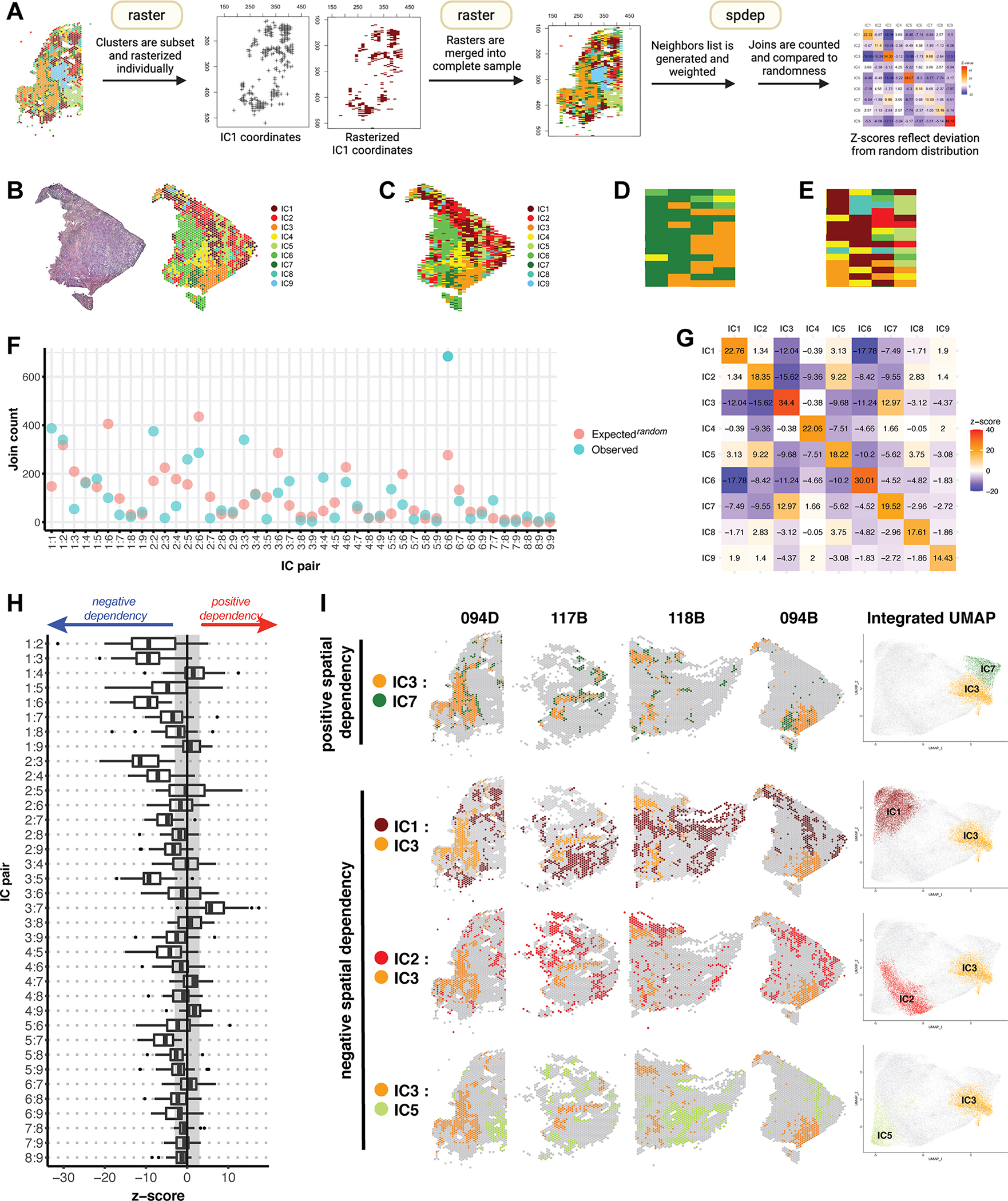
Figure 5. Spatial analytics of integrated clusters reveals a consistent molecular topography.

(A) An overview of join count analysis (JCA). Each sample is subset by integrated cluster (IC), and corresponding coordinates are rasterized individually using R package raster. Subsetting allows each IC to be coded uniquely during rasterization. Individual rasters for all 9 ICs are then merged to recreate the complete sample. R package spdep is then used to generate a neighbors list with spatial weights for each observation. Join counts for all cluster pairs are then tabulated and compared to a spatially random distribution. (B) Mapping of ICs on sample 094B. (C) Raster of sample 094B, in which each spatial feature is represented by a pixel coded by IC assignment. (D) A region of sample 094B representative of clustering, in which any given pixel is likely to have a similar group of neighbors. (E) A region representative of dispersion, in which most pixels have dissimilar neighbors. (F) JCA results for sample 094B. For each IC pair, the observed join count is indicated, along with what would be expected under conditions of spatial randomness. (G) Z-values corresponding to the analysis in (F), reflecting the deviation of the observed join count from theoretical randomness. A positive z-value indicates spatial clustering, a negative value indicates spatial dispersion, and a value close to 0 indicates no spatial dependency, i.e. a near random distribution. (H) A summary of z-values resulting from JCA of all 28 samples represented in a box plot. The box represents the interquartile range, with the median marked by a vertical line. Outliers are represented by points outside the range of the whiskers. The shaded region represents our selected z-value cutoff of +/−3 (as described in Methods) to assess significance of results. All autocorrelations were strongly positive (z ≥ 10) and are not represented here. (I) Spatial mapping and UMAP embeddings of selected IC pairs found to trend towards positive and negative spatial dependency.
