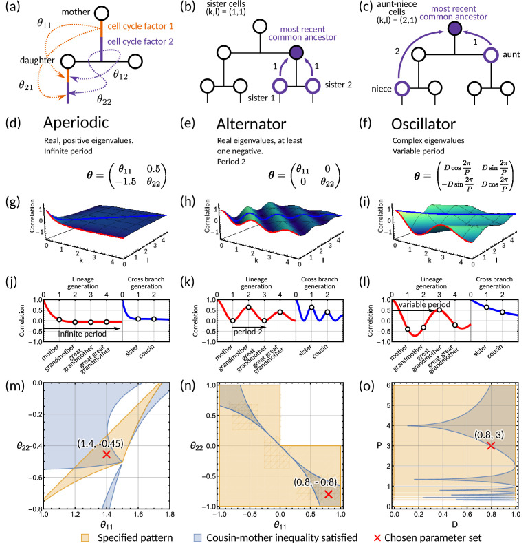
Figure 2. Analysis of the inheritance matrix model identifies three distinct lineage tree correlation patterns.

(a) Diagram illustrating the inheritance matrix model with two cell cycle factors which affect the interdivision time of a cell. Each factor in the mother exerts an influence on a factor in the daughter through the inheritance matrix $\mathit{\theta }$. (b,c) Schematics showing how the coordinate $(k,l)$ introduced in ‘The inheritance matrix model reveals three distinct interdivision time correlation patterns’ is determined. This coordinate describes the distance to the most recent common ancestor for chosen pair of cells. Examples shown are (b) sister pairs with $(k,l)=(1,1)$, and (c), aunt-niece pairs with $(k,l)=(2,1)$. (d-o) Panels demonstrating the three correlation patterns that arise from the inheritance matrix model with two cell cycle factors. (d-f) Example inheritance matrices $\mathit{\theta }$ that produce the desired patterns: (d) aperiodic, (e) alternator and (f) oscillator correlation patterns. (g–i) Three-dimensional plot of the generalised tree correlation function (Equation M3) demonstrating each of the three patterns. On each plot we highlight the lineage generation correlation function ($k=0$ or $l=0$) (red line) and the cross-branch generation correlation function ($k=l$) (blue line). The shading of the 3D plot indicates the correlation coefficient at that point on the surface. (j–l) The lineage and cross-branch generation correlation functions plotted individually, showing the different dynamics for each pattern. (m–o) Region plots showing parameter values where the relevant pattern is obtained (orange) and where the cousin-mother inequality is satisfied (blue) for the $\mathit{\theta }$ matrices given in panels (d-f). White bands on (o) indicate where $P=\frac{2}{k}$ which results in real eigenvalues and therefore does not produce an oscillator pattern. Within the parameter region that both produces the desired pattern and also satisfied the cousin-mother inequality, we choose a parameter set (red cross) which is used for the corresponding plots in the panels above. In all panels we fix $\mathit{\alpha }={(1,1)}^T$ and the noise vector $\mathit{z}$ to have covariance equal to the identity matrix.