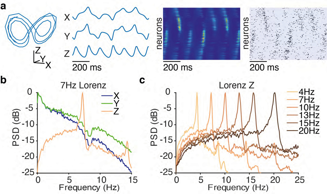
Extended Data Fig. 1. Simulation of Lorenz system at different speeds.

This figure illustrates the underlying dynamical system used for the simulation experiments. (a) An example Lorenz trajectory in a 3-dimensional state space (far left) and with three dynamic variables plotted as a function of time (middle left) for a system with Z-oscillation peak frequency of 7 Hz (i.e., the power spectrum of the Lorenz system’s Z-dimension had a pronounced peak at 7 Hz). Firing rates for the simulated neurons were computed by a linear readout of the Lorenz variables followed by an exponential nonlinearity (middle right). Spikes from the firing rates were then generated by a Poisson process (far right). The example trial shown here is identical to “Trial 2” in Fig. 2a, but with a wider plotting window. (b) Power spectrum of the individual Lorenz variables for the system with a Z-oscillation peak frequency at 7 Hz. Because only the Z variable has a clear peak in the power spectrum, this variable was used exclusively for all further analyses in simulations except Supp. fig. 1. (c) Power spectrum of the Z dimension for Lorenz systems simulated with different Z-oscillation peak frequencies.