
Figure 8:
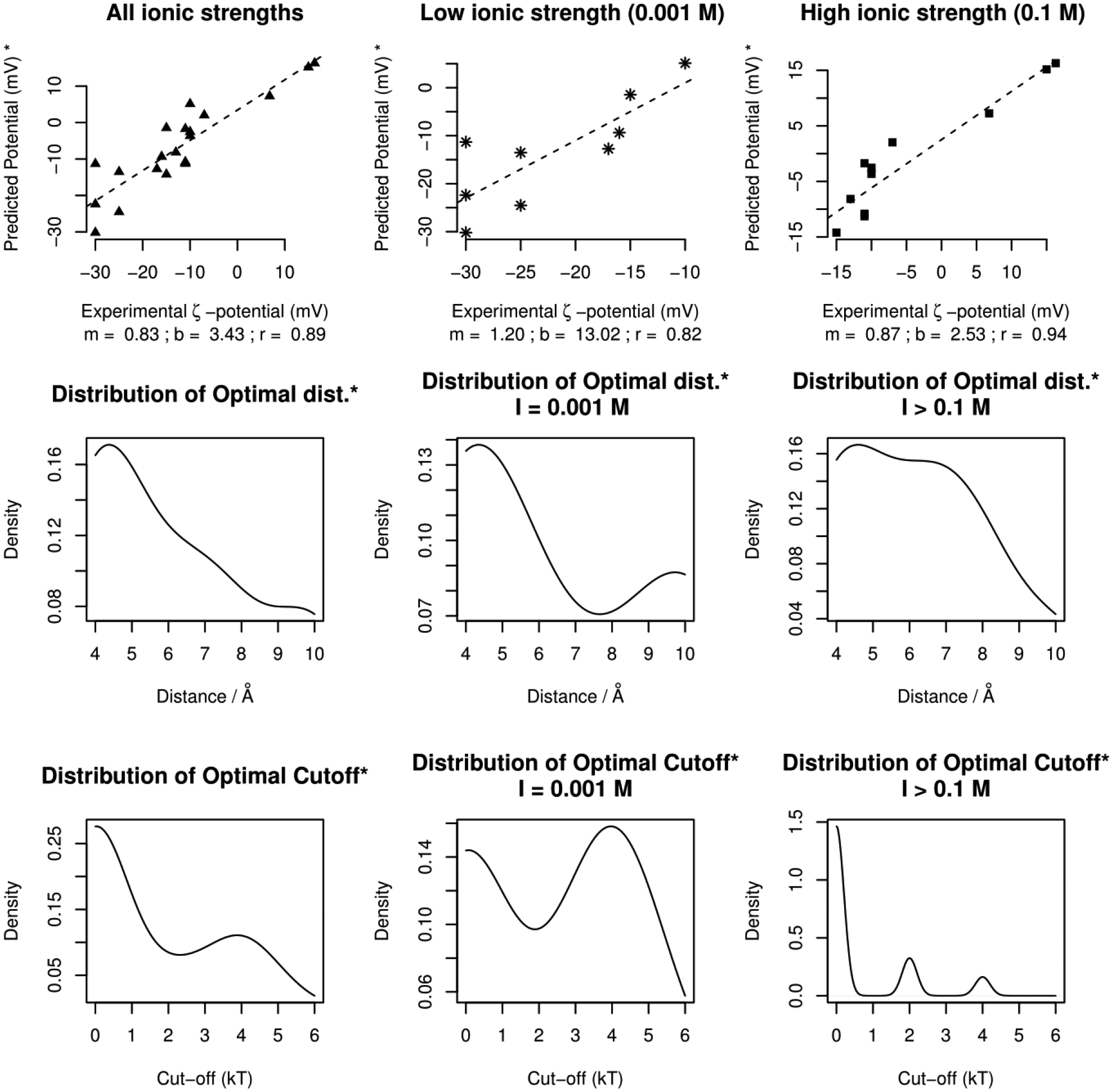
Top Panel – The correlation plots (slope = m, y-intercept = b, correlation = r) for the best predicted potential. The plots in the center and far right combine to produce the one in the far left. Bottom Panel – the corresponding density distribution of optimal cut-offs.