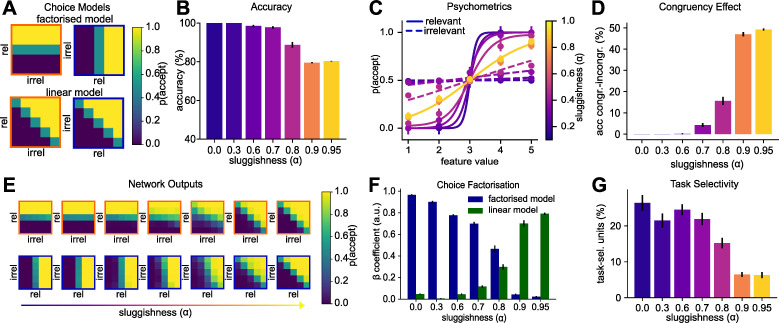
Fig 3. Modelling the cost of interleaving with a “sluggish” task signal.

(A) Illustration of the cost of interleaved training. The factorised model (top) assumes that two separate category boundaries are learned, one for each task. The linear model (bottom) assumes that the task signal is ignored, leading to the acquisition of a diagonal category boundary that yields high performance on both tasks. We hypothesised that interleaved training would promote a solution as predicted by the linear model. (B) Test phase accuracy of neural networks trained on interleaved data with different levels of “sluggishness” (exponential average of the task signal). The higher the sluggishness, the lower the task accuracy. (C) Sigmoidal curves fit to the choices of networks described in (B). The solid lines indicate how the choices depend on the relevant dimension and the dashed line how they depend on the irrelevant feature dimension. As the sluggishness increases, sensitivity to the relevant dimension decreases and to the irrelevant dimensions increases. (D) Difference in accuracy between congruent and incongruent trials (i.e., those with the same or different responses across tasks). The congruency effect depends on the amount of sluggishness. (E) Network outputs (choices) for different levels of sluggishness. As sluggishness increases, the networks move from learning a “factorised” to learning a “linear” solution. (F) Linear regression coefficients obtained from regressing the outputs shown in (E) against the models shown in (A), confirming that sluggishness controls whether a factorised or linear solution is learned. (G) Proportion of units in the hidden layer which are task selective. With increasing sluggishness, fewer units are exclusively selective for one task.