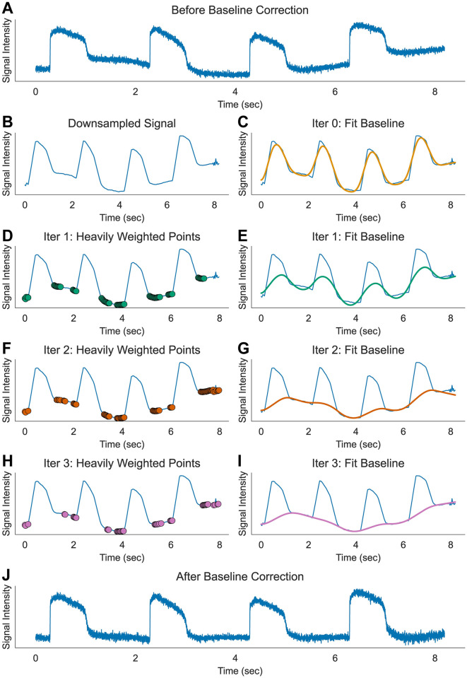
Fig 5. Baseline correction.
(A) Sample raw trace of AP from single pixel with baseline drift before correction. Dye bleaching and fluctuation from perfusion flow may cause slow drift in baseline. (B-I) Iterative method of polynomial fitting for baseline estimation using asymmetric least squares method. Step 1: Resample the original signal to lower time resolution to accelerate calculation (here, 128 points are sampled from 8192 points, panel B). Step 2: Fit the signal with least squares polynomial fitting (here 3rd order, panel C). Step 3: Apply reduced weight when the signal is above the polynomial fitting by multiplying asymmetric parameter p (here 0.001, panel D). Step 4: Apply polynomial fitting again and repeat adjusting weight (panel E). Step 5: repeat iteration until the baseline estimation converges (panel F-I). (J) Sample trace after 5 iterations of baseline correction.

