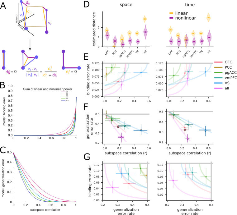
Figure 3.
Formalizing subspace structure through a geometric theory of binding and generalization for neural codes. A. Schematic of the geometric decomposition. (top) The representation from Figure 2 is decomposed into linear dL (yellow) and nonlinear dN (purple) components. (bottom) The relative length of these components determines the subspace correlation from before: dN = 0 and dL > 0 implies perfect subspace correlation (bottom left), both dN > 0 and dL > 0 implies intermediate subspace correlation (bottom middle), and dN > 0 while dL = 0 implies zero subspace correlation (bottom right). B. The relationship of the binding error rate predicted by our theory with subspace correlation. The different lines are codes with different sums of squared linear and nonlinear distances. The line is created by varying the tradeoff between linear and nonlinear distance such that the sum remains constant. The left side of the line is when linear distance is zero and nonlinear distance is the total distance; the right side is the opposite extreme. C. The same as B but for the generalization error rate. D. (left) The nonlinear and linear distances estimated for the left and right value codes within each brain region. (right) The same as on the left, but for the offer 1 and offer 2 value codes. The violin plot shows the distribution of bootstrap resamples. E. The predicted binding error rate as a function of subspace correlation for each region, derived from the distance estimates in D. The left-right plot convention is the same as in D. The gray line shows the chance level of binding errors. F. The predicted generalization error rate as a function of subspace correlation for each region, derived from the distance estimates in D (for the open circles) and computed empirically with a linear decoder (for the outlined circles). The gray line is the chance level. The left-right plot convention is the same as in D. G. Each region shown on the plane defined by the generalization and binding error plane, derived from the distance estimates in D. The gray lines are the chance levels for each of the error types. The left-right plot convention is the same as in D.

