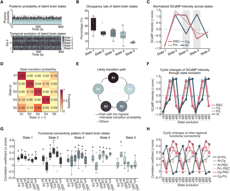
Fig. 4. Spatiotemporal properties of latent brain states during the resting-state condition.

(A) Top: Time-varying posterior probabilities of the brain states identified by the BSDS model. Bottom: Temporal evolution of the identified brain states. (B) Occupancy rates of the latent brain states. The occupancy rate of State 1 was the highest across the brain states. Data are presented as box and whisker plots, where boxes encompass values between the 25th and 75th percentiles, and horizontal lines represent median values. Dots in the figure represent correlation coefficients for each individual rats. (C) Normalized GCaMP activities of AI, Cg, PrL, and RSC across latent brain states. Cg, PrL, and RSC showed coupled activities across all the states whereas the activity of AI showed coupling and decoupling with activities of Cg, PrL, and RSC. (D) Dynamic switching properties of latent brain states. State switching probability, defined as the probability that a latent brain state at time instance (t) stays in its own state or switches to other states at time instance (t + 1). (E) Analysis of likely switching paths revealed that state transition follows a cyclic pattern. (F) Evolution of GCaMP activities of four regions following the likely transition path identified in Fig. 4E. Evolution of GCaMP activity exhibits a cyclic pattern with coupling and decoupling between AI and other regions. (G) Functional connectivity pattern between regions for each latent brain state. Data are presented as box and whisker plots, where boxes encompass values between the 25th and 75th percentiles, and horizontal lines represent median values. Dots in the figure represent the correlation coefficients from each individual rat. *P < 0.01, n = 7, two-tailed t test, FDR-corrected. (H) Evolution of inter-regional functional connectivity (Fisher z-transformed partial correlation coefficient) following the likely transition path identified in Fig. 4E.