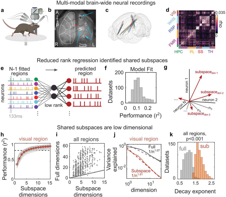
Figure 1. Interactions between brain regions are organized into subspaces.

(a) Schematic of experiments combining neural recordings from four Neuropixels probes across cortical and subcortical regions and simultaneous widefield calcium imaging of neural activity across dorsal cortex. (b) Field of view of widefield imaging showing the dorsal cortex and four craniotomies with implanted electrodes (thin gray shadows; indicated by blue arrows). Dotted white lines outline general cortical regions (see Fig. S1 for parcellation). R and L denote animal’s right and left. (c) Reconstructed probe locations from six recordings in three mice; colors indicate mice. (d) Correlogram showing correlation between pairs of cells within a brain region compared to pairs across regions for an example recording. Color bars along axes correspond to brain regions, held constant throughout figures. (e) Schematic of reduced rank regression to predict activity of each neural population. Spontaneous spiking activity was binned to 133ms windows, and the evoked response was removed (see methods). The moment-to-moment spiking variability of one region was predicted using spiking variability of all other regions. (f) Cross-validated predictive performance of all regression models (models fit to n=630 datasets, see methods). (g) Schematic of the shared subspace, showing that the subspace is spanned by a set of dimensions within the neural activity of the predicted region that are correlated with neural activity in other regions. (h-i) A small subspace of neural activity within a region was shared with other regions. (h) Gray lines show cumulative percent of the explainable variance captured by each dimension of the reduced rank regression model (see methods). Red line shows mean performance. Gray lines show cross-validated performance from n=84 datasets. Black dotted line shows 80% of explainable variance. (i) Comparison between the number of subspace dimensions and the number of ‘local’ dimensions needed to explain 80% of the explainable variance within a region. Local dimensionality was estimated with a cross-validated measure²², which revealed that 24.1 dimensions (CI: 23.0–25.4) were needed to capture 80% of the explainable variance within each region. Dots show individual datasets (n=630). Dotted line shows unity. (j) Example results from visual cortex comparing the decay in the variance explained by each additional subspace or local dimension. Solid line and shaded regions show mean and SE, respectively (n=84 model fits). Dotted lines show fit of power law. (k) Histogram of power law exponents from fits to full (grey) and subspace (red) dimensionality across all regions (n=630 datasets).