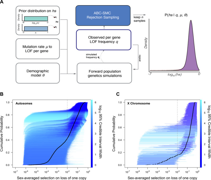
Figure 1. Estimating hs for loss-of-function (LOF) across human genes.

(A) Schematic of the approach to infer heterozygous selection coefficients (hs) for each gene. We assume prior distributions log₁₀(s)~U(–6,0) and h~U(0,1). We further assume a mutation rate μ to LOF alleles per gene and a demographic model specified by parameters $\theta$, which describe changes in the effective population size N_e at time points in the past. These parameters are used in forward population genetic simulations based on a Wright–Fisher model of selection (see 'Materials and methods'). For each iteration i, the simulation generates a frequency q_i of LOF alleles, which is then compared to the observed LOF frequency q for a given gene. The proposed value of (hs)_i is retained if within a tolerance ε, which is decreased over time, or rejected otherwise. For each ε, this procedure is repeated until there are 50,000 acceptances, providing a sample from the posterior distribution of the probability of hs given the observed frequency q of LOF variants for a gene (as well as the mutation rate and demographic model). (B) The cumulative distribution of the estimated heterozygous selection coefficient hs for each autosomal gene. Black dots represent the point estimate of hs for each gene, based on the maximum a posteriori estimate (i.e., the mode) of the posterior distribution. Horizontal lines represent the 95% credible intervals for each gene and are colored according to the width of the interval on a log₁₀ scale. (C) A similar plot, but for non-pseudoautosomal region (PAR) X-linked genes, with sex-averaged selection on the loss of a copy on the X calculated as the average of s and hs (see 'Materials and methods').