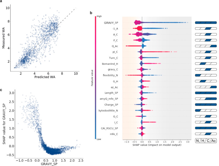
Figure 3.

Model explanation. (a) Predictions of the trained RF regressor model on the test set. On the ordinate, WA values for SPs belonging to the test set and measured with the NLR-based amylase assay are reported; on the abscissa, their WA values predicted with the trained RF model are displayed. Note that measurements and prediction show a high degree of agreement with a calculated MSE of 1.22 WA, thus indicating a good performance of the generated RF model. The dashed line represents the ideal situation where all predicted and measured values would align. (b) SHAP summary plot of the 20 most impactful features: GRAVY_SP, overall SP hydrophobicity; –1_A, Ala at −1 of the AxA cleavage site; A_C, frequency of Ala in the C-region; P_C, frequency of helix-breaking Pro in the C-region; Q_Ac, frequency of glutamine in the Ac-region; pI_C, pI of the C-region; Turn_C indicates a helix-breaking residue at the end of the H-region; Bomanlnd, protein–protein interaction in the SP; Gravy_C, hydrophobicity of the C-region; Flexibility_N, measure for flexibility and charge in the N-region; G_H, frequency of Gly in the H-region; Ez_Ac, potential for Ac-region insertion in lipid membranes; Length_SP, overall length of the SP; amyQ_mfe_SP, minimum folding energy of the RNA secondary structure encoded by the sp-amyQ gene fusion; Charge_SP, charge of the SP; Kytedoolittle_N, hydrophobicity of amino acids in the N-region; G_C, frequency of Gly in the C-region; I_C, frequency of Ile in the C-region; CAI_RSCU_SP, codon adaptation index of the SP; Mfe_C, minimum folding energy of the RNA secondary structure in the C-region-encoding sequence (for full descriptions, see Supporting Information Table S2). A high dispersion of SHAP values on the abscissa indicates a broad effect of the respective feature on the model. Each data point represents a specific SP, the color of the data point indicates the value of that feature in the feature-specific scale, and the position on the abscissa indicates the SHAP value for that particular feature. SHAP values for the whole data set sum up to the base value of the model (4.45 WA, average model output calculated over the 4421 selected SPs). Positive SHAP values indicate a negative impact on the model outcome and vice versa. Cartoons on the right highlight the corresponding SP parts of each particular feature. (c) SHAP-dependence plot for “GRAVY_SP”, which is a two-dimensional representation of the information summarized by the first line of panel b. The GRAVY index is represented on the abscissa: negative values indicate low hydrophobicity, and positive ones indicate high hydrophobicity. On the ordinate, SHAP values are displayed: negative values indicate a beneficial effect on protein secretion, and positive ones indicate a detrimental effect. Vertical dispersion of SHAP values for similar GRAVY indexes can be explained through the interaction effect between features (described by SHAP interaction values, summarized in Supporting Information Figure S7 and Supporting Information Figure S8). To exemplify, the high variability visible in the negative range of the GRAVY index is to be attributed mainly to the feature “–1_A” (Supporting Information Figure S6). The data imply that a very low hydrophobicity will have a strong negative impact on protein secretion, while a GRAVY index value of around 1.0 will be most favorable for protein secretion.