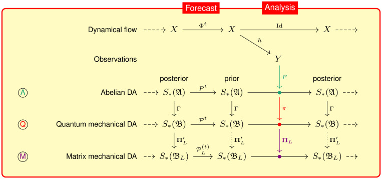
Fig. 1.

Schematic representation of the abelian and nonabelian formulations of sequential data assimilation (DA), showing a forecast–analysis cycle. The Top row of the diagram shows the dynamical flow Φ^t : X → X. The second row shows the observation map h : X → Y used to update the state of the DA system in the analysis step. The rows labeled , , and show the abelian, infinite-dimensional nonabelian (quantum mechanical), and finite-dimensional nonabelian (matrix mechanical) DA systems, respectively. In , the forecast step is carried out by the transfer operator $P^t:S_{\ast }(\mathfrak{A})\to S_{\ast }(\mathfrak{A})$ acting on states of the abelian algebra $\mathfrak{A}$. The analysis step (green dot) is represented by an effect-valued map $F:Y\to \mathfrak{A}$ that updates the state given observations in Y. In , the forecast step is carried out by the transfer operator ${\mathcal{P}}^t:S_{\ast }(\mathfrak{B})\to S_{\ast }(\mathfrak{B})$ acting on states of the nonabelian operator algebra $\mathfrak{B}$. The analysis step (red dot) is carried out by an effect $\mathcal{F}:Y\to \mathfrak{B}$ given by the composition of F with the regular representation π of $\mathfrak{A}$ into $\mathfrak{B}$ (red arrow). The state space $S_{\ast }(\mathfrak{A})$ is embedded into $S_{\ast }(\mathfrak{B})$ by means of a map Γ, which is compatible with both forecast and analysis; Eqs. 4 and 9. This compatibility is represented by the commutative loops between and having Γ as a vertical arrow. To arrive at the matrix mechanical DA, , we project $\mathfrak{B}$ into an L²-dimensional operator algebra ${\mathfrak{B}}_L$ using a positivity-preserving projection ${\mathbf{\Pi }}_L$. The composition of this projection with ℱ leads to an effect ${\mathcal{F}}_L:Y\to {\mathfrak{B}}_L$ employed in the analysis step (purple arrow and dot). Moreover, ${\mathbf{\Pi }}_L$ induces a state space projection $\mathbf{\Pi }{\prime }_L:S_{\ast }(\mathfrak{B})\to S_{\ast }({\mathfrak{B}}_L)$ and a projected transfer operator ${\mathcal{P}}_L^{(t)}:S_{\ast }({\mathfrak{B}}_L)\to S_{\ast }({\mathfrak{B}}_L)$ employed in the forecast step. Vertical dotted arrows indicate asymptotically commutative relationships that hold as L → ∞.