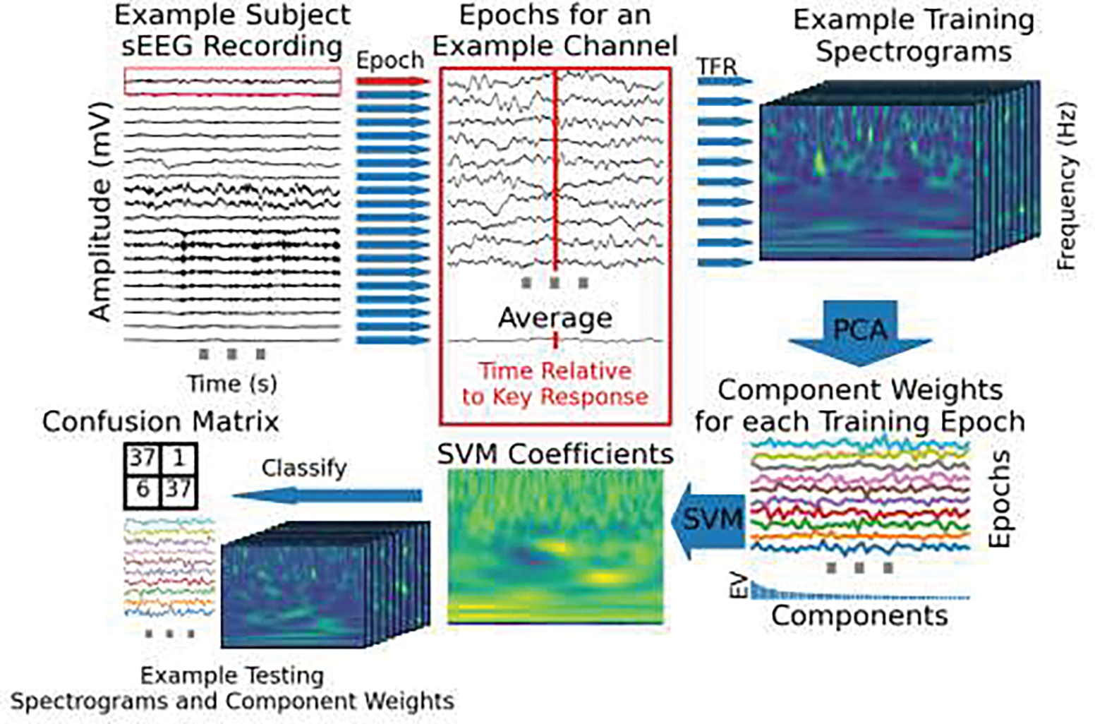
Figure 1.

a) The task schema is shown per trial. The diagram is to scale in time. A typical response time (RT) is shown in red. Gray vertical lines indicate different time lengths used for that event to make trials unpredictable for the participant. Trials were included if the response was correct and the response time was within the cue period. b) A schematic of the SVM analysis process is shown. This procedure is repeated for each sEEG contact individually. First (labeled 1), the epochs are created for each of the shaded time areas in a. Example data from the response epoch is shown. Then (2), each epoch is decomposed into time-frequency (TFR) space. Next, principal component analysis (PCA) is applied to the spectrograms for training trials so each trial can be represented by weights per component (3). The explained variance (EV) of the components for this example is shown in the bar plot beneath the PCA weights per component. Next, a support vector machine (SVM) is fit to the PCA weights per trial. The SVM coefficients are shown both in relation to the component weights (4 top) and multiplied by the principal components and summed, projecting back into the time-frequency domain (4 bottom). Lastly, the coefficients are multiplied and summed with the component weights from each test trial and classified based on which category (movement or rest) the output is closer to. The linear decision boundary for the first two principal components out of the 50 used is shown for this example (5). c) The first three eigenvector spectrograms from the PCA decomposition for this example contact. Each principal component is a matrix of time-frequency loadings. Each trial was represented as a vector of weights, one for each principal component, that the SVM used to learn a decision boundary. The dimensionally-reduced, time-frequency representation of each trial can be visualized as a sum of these eigenvector spectrograms weighted by the vector of principal component weights for that trial. The SVM coefficients representing the optimal separation between response and inter-trial spectrograms are represented this way in step 4 (bottom) in b which creates a response-spectrogram-matching-template.