Figure 7.

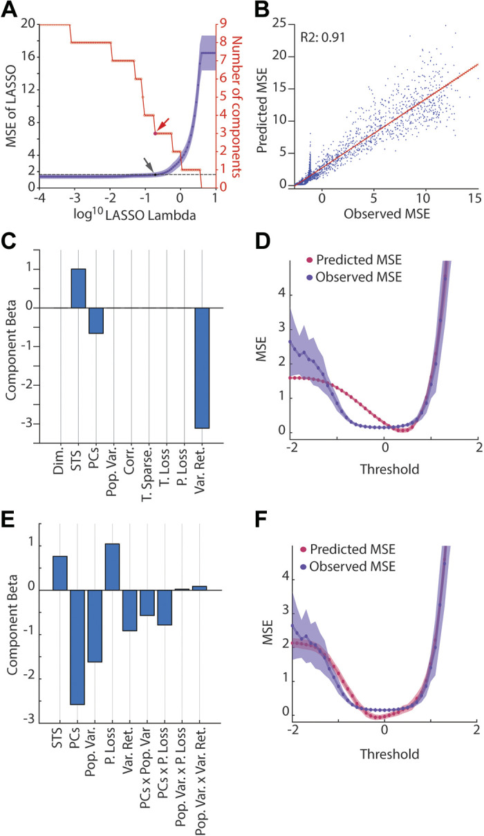
Relationship between GCL population statistics and MSE. A: LASSO regression was used to identify GCL population metrics that predicted learning performance. A: the model selection as a function of progression of the Lambda parameter (which is the penalty applied to each regressor). The following potential regressors were used: dimensionality (Dim.), spatiotemporal sparseness (STS), explanatory principal components of the GC population (PCs), population variability (Pop. Var.), spatial sparseness (S. Sparse.), temporal sparseness (T. Sparse.), temporal lossiness (T. Loss.), population lossiness (P. Loss), and input variance retained (Var. Ret; Fig. 5). Arrow shows selection point of LASSO regression MSE using “1SE” (1 standard error) method (see methods, purple lines, black dot, and arrow indicating the selected model, with red arrow showing selection point in the parameter reduction plot, red). B: relationship between LASSO model (predicted relative MSE) against the observed relative MSE (ratio of GC MSE to MF alone MSE) with fit line and variance explained by regression (R² = 0.91). C: regression slopes of the selected LASSO model from A, showing that STS, PCs, and input variance retained are the selected regressors, with Var. Ret. being the largest contributing factor. All factors normalized to a normal distribution for comparison. D: the output of the selected model and the observed MSE plotted against threshold for a comparison of fits, demonstrating high accuracy in the 0–2 range, but less accuracy in the −2 to 0 range. E and F: similar to C and D except using Bayesian information criteria stepwise regression model to select metrics that explain learning. GCL, granule cell layer; MSE, mean squared error.