Roelants et al. 10.1073/pnas.0608378104. |
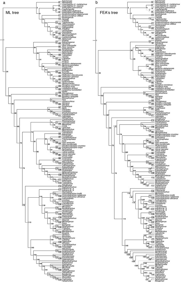
Fig. 3. Phylogenetic topologies used to calculate timetrees for living amphibians. (a) Unconstrained ML tree (-lnL = 128,388.19). Node labels are cross-referenced in SI Data Set 1. (b) ML tree constrained to be compatible with the study of Frost et al. (1) (FEA's tree; -lnL = 128,873.46). Nodes with labels ending with "f" are in conflict with the unconstrained tree. Unconstrained and terminal branches not included in the backbone constraint are colored gray.
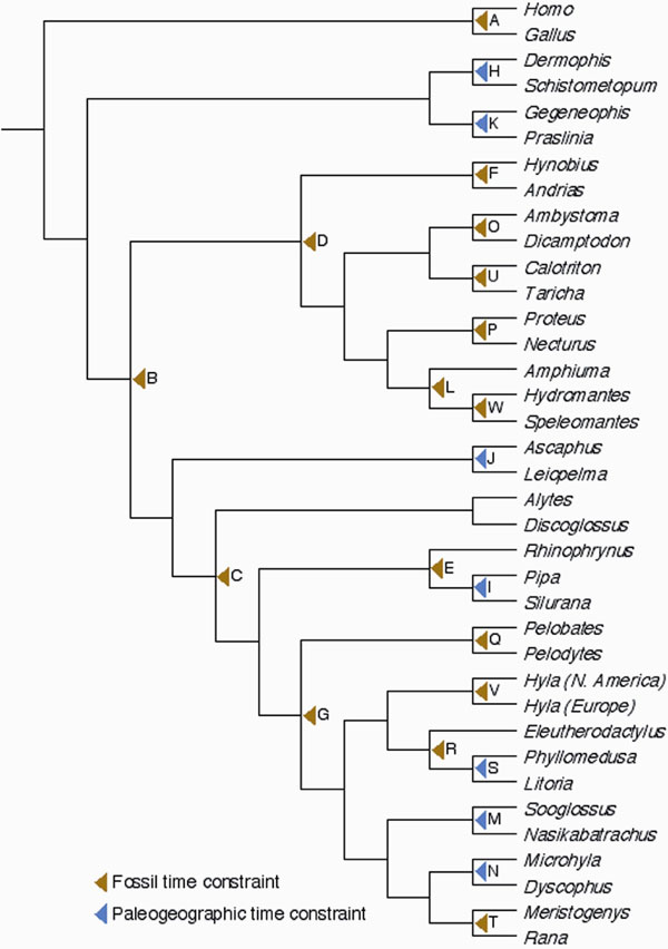
Fig. 4. Pruned 38-taxon topology used for evaluating the sensitivity of our dating analyses to exclusion of calibration points, and change of relaxed clock model priors.

Fig. 5. Schematic representation of the clade-specific net diversification rates estimated prior (presplit) and posterior (postsplit) to the earliest node of each clade in the timetree. The ratio of the latter over the former represents a measure for the acceleration.

Fig. 6. Effect of excluding individual calibration points on the resulting divergence time estimates. Negative values represent average age reductions, positive values represent average increases. Letters refer to excluded calibration points and correspond to SI Fig. 4 and SI Table 2. (a) Absolute mean difference in divergence age (Myr). (b) Relative mean difference in divergence age (%).
SI Text
Detailed Description of Methods and Results
1. Phylogeny Reconstruction
1.1 Data set composition
We compiled a multigene data set for 171 amphibian ingroup species, including 120 frogs, 27 salamanders, and 24 caecilians (see SI Table 1). Amphibian taxonomy is currently in a state of flux, but this study follows the classification of Frost et al.'s (henceforth referred to as FEA) recently published 'Amphibian Tree of Life' (1), which is based on the largest body of phylogenetic evidence hitherto published. Because FEA's taxonomy differs markedly from previously proposed classifications, we also make reference to Dubois' 'Amphibia mundi' (2), which retains more consistency with long-established systematic arrangements.
Because our taxon sampling is focused on a maximal taxonomic diversity at higher taxon level, net diversification rates will be increasingly underestimated toward the present, and within subfamilies. To reduce this effect in species-rich (sub)families, we attempted to include at least two representatives that span their basalmost split according to previous phylogenetic studies (1, 3-16). Given convincing molecular support for the monophyly of living amphibians with respect to amniotes (17-19), we sampled two mammals (Homo sapiens and Mus musculus), a bird (Gallus gallus) and a lizard (Lacerta lepida) to constitute the outgroup for phylogeny inference.
The data set is a concatenation of one mitochondrial gene fragment (»550 bp of the 16S rRNA gene) and four nuclear protein-coding gene fragments (»675 bp of CXCR4, »1285 bp of NCX1, »550 bp of RAG1, and »1123 bp of SLC8A3). Sequences of two teleost fishes (16S rRNA, CXCR4, RAG1 and SLC8A3 of Danio rerio and NCX1 of Oncorhynchus mykiss) were combined to obtain a single chimeric outgroup taxon for the dating analyses. DNA sequences for many taxa were sourced from previous studies performed by the authors (16, 20-22). The mammal, bird and fish sequences were retrieved from GenBank (SI Table 3). Additional amphibian sequences as well as those of Lacerta lepida were newly obtained via whole genome DNA extraction, PCR-amplification and cycle-sequencing. PCR reactions were performed with FastStart TaqDNA Polymersae (Roche) in total volumes of 25 ml, using the following cycling conditions: (i) initial denaturation for 240s at 94°C, (ii) 36 cycles with denaturation for 40s at 94°C, annealing for 60s at 55°C, and elongation for 60s at 72°C, and (iii) final elongation for 120s at 72°C. Annealing temperatures for fragments of NCX1 were 50-52°C. Relevant primer sequences are listed in SI Table 4 or published elsewhere (20-22). Weakly amplified or problematic PCR-products were cloned into a pGEM-T Easy vector (Promega) and submitted to an additional PCR reaction. Well-amplified PCR-products were purified via gel extraction (Qiagen), cycle-sequenced along both strands using the BigDye Terminator v3.1 Cycle Sequencing kit and visualized on an ABI Prism 3100 Genetic Analyzer (Applied Biosystems)
Individual alignments of all fragments were created with ClustalX 1.81 (23) and manually corrected with MacClade 4.06 (24). Exclusion of 527 ambiguously aligned positions in the periphery of indels resulted in a total matrix length of 3747 bp (16S rRNA: 369 bp, CXCR4: 586 bp, NCX1: 1207 bp, RAG1: 486 bp, SLC8A3: 1099 bp).
1.2. Phylogenetic analyses
Phylogenetic analyses were performed with the GTR+G+I model of DNA evolution, identified as the best-fitting model under the Akaike information criterion implemented in Modeltest 3.0.6 (25). Maximum likelihood (ML) analyses involved preliminary heuristic searches with optimized model parameters using Phyml 2.4.1 (26). The resulting tree was entered into PAUP* 4.0b10 (27) and submitted to additional rounds of TBR branch swapping, with fixed model parameters estimated from the starting tree. Clade support under ML was assessed by 1000 replicates of nonparametric bootstrapping (BS), performed with Phyml. Bayesian posterior probabilities (PP) were estimated using Mrbayes 3.1.2 (28), under a mixed GTR+G+I model partitioned over the different gene fragments, with flat dirichlet priors for base frequencies and substitution rate matrices, and uniform priors for among-site rate parameters. Two parallel MCMC runs of four chains each were performed (one cold and three heated, temperature parameter = 0.2), with a length of 6,000,000 generations, a sampling frequency of one per 1000 generations and a burn-in corresponding to the first 1,000,000 generations. Convergence of the runs was confirmed by split frequency standard deviations (<0.01), and by potential scale reduction factors (~1.0) for all model parameters.
Despite a high overall resemblance, our ML tree (SI Fig. 3a; -lnL = 128388.19) shows several alternative arrangements compared to FEA's proposed amphibian tree (1). To investigate the effect of these differences on amphibian divergence time estimates, we constructed an alternative phylogenetic hypothesis, by heuristic ML searches with PAUP*, using a backbone constraint compatible with FEA's tree. The resulting topology (-lnL = 128873.46) is shown in SI Fig. 3b.
Our analyses lend robust support to the 'Batrachia' hypothesis (17, 19, 29), i.e., Gymnophiona being the sister-clade of (Anura + Caudata) (BS = 93%; PP = 1.0). Within Gymnophiona, the hierarchy of inter-family divergences is resolved in full agreement with recently proposed phylogenetic hypotheses (29-31), with the South American Rhinatrematidae as the earliest diverging family (BS = 99%; PP = 1.0), and an Asian clade combining Uraeotyphlidae and Ichthyophiidae (BS = 100%; PP = 1.0) as the subsequent sister-clade of all remaining caecilians (BS = 100%; PP = 1.0). Unlike in previous studies (1, 32), we find Scolecomorphus, rather than Herpele + Boulengerula as the next diverging branch. Our analyses robustly confirm previous evidence that Caeciliidae as defined traditionally (i.e., excluding Typhlonectinae) represent a paraphyletic assemblage (5, 31), with an African clade combining (Herpele + Boulengerula) as the sister-group of all other caeciliids + Typhlonectinae (BS = 100%; PP = 1.0), and the type genus Caecilia as the closest relative of Typhlonectinae (BS = 100%; PP = 1.0).
In Caudata, our phylogenetic hypothesis bears high similarity with the phylogeny proposed by Wiens et al. (33) based on combined ribosomal and RAG1 sequences, challenging a previously postulated alliance of the paedomorphic families Amphiumidae, Proteidae and Sirenidae based on morphological data (34) or of Proteidae and Sirenidae based on molecular data (1). Instead, we recover a basal split between Cryptobranchoidea (Hynobiidae + Cryptobranchidae; BS = 100%; PP = 1.0) and a modestly supported clade combining Sirenidae with all remaining salamanders (BS = 62%; PP = 1.0). As a primary difference with the studies of Wiens et al. and Frost et al. (1, 33), our analysis suggests the strong association of Proteidae with the assemblage of Rhyacotritonidae, Amphiumidae and Plethodontidae (BS = 91%; PP = 1.0), rather than with Ambystomatidae and Salamandridae. Our analyses fail to provide a robust hypothesis for plethodontid relationships, but the inferred relationships are congruent with recent molecular results based on complete mitochondrial (6, 35) or nuclear gene sequences (11).
In Anura, our analyses provide increased support for a paraphyletic hierarchy of archaeobatrachian divergences (1, 21, 29, 36, 37), challenging the monophyly of archaeobatrachian frogs as recovered by previous neighbor-joining and parsimony analyses of ribosomal DNA (18, 38), or the basal origin of Pipoidea, as supported by combined larval and adult morphological data (39, 40). They further confirm the existence of five major neobatrachian lineages: (i) Heleophryne, (ii) Sooglossus + Nasikabatrachus, (iii) Myobatrachidae + Caudiverbera (Australobatrachia sensu (1)), (iv) Nobleobatrachia [Hyloidea sensu (20, 29, 37, 41)], and (v) Ranoides [Ranoidea sensu (2, 8, 9, 37)]. Within Nobleobatrachia, polyphyly of Hylidae and Leptodactylidae as previously defined (2), is reaffirmed (1, 36, 41-43). The sister-clade relationship of Neotropical Phyllomedusinae and Australian/New Guinean Pelodryadinae (1, 36, 41-43) is confirmed (BS = 100%; PP = 1.0), which is important for our divergence time estimations. The existence of a clade combining the leptodactylid frog genera (Leptodactylus, Physalaemus and Pleurodema) is supported by a unique molecular apomorphy in the NCX1 gene, corresponding to the insertion of two amino-acids. Within Ranoides, we find moderate bootstrap and strong Bayesian support for the pairing of Microhylidae with the African endemic Afrobatrachia (1, 9, 36), the latter including Hemisotidae, Brevicipitidae, Arthroleptidae and Hyperoliidae (BS = 80%; PP = 1.0). Within Microhylidae, we find modest support for the pairing of the Madagascan Scaphiophryne with the South American genus Synapturanus (BS = 60%; PP = 0.99) and strong support for the pairing of Madagascan Dyscophus with Asian Microhylinae (BS = 96%; PP = 1.0). These results contrast with FEA's tree (1), which recovered sister-clade relationships between Dyscophus and Australian/New Guinean Asterophryinae and between Scaphiophryne and Microhylinae. Within Natatanura, our analyses confirm the existence of a large African endemic clade (1, 8). However, unlike FEA's tree, this clade does not include the Indian endemic genus Indirana.
2. Timetree Estimation
2.1 Dating methods
The hypothesis that our data evolved according to a strict molecular clock is strongly rejected by a c2 likelihood ratio test (C 2 = 1896.48; df = 174; P ~ 1.10-29). We therefore performed dating analyses using two different relaxed molecular clock methods, which have recently been demonstrated to be the least sensitive to taxon sampling (44), and which have complementary advantages and limitations. Thorne & Kishino's (TK) method (45) accommodates unlinked rate variation across different loci (a 'multigene' approach), allows the use of time constraints on multiple divergences, and uses a Bayesian MCMC approach to approximate the posterior distribution of divergence times and rates, but uses an F84+G model (or a nested variant) for branch length estimation, and fails to incorporate phylogenetic uncertainty in the posterior distribution. Sanderson's penalized likelihood (PL) method (46) allows branch length estimation using more complex DNA substitution models (e.g., GTR+G+I) and the use of a posterior tree set to estimate credibility intervals (CI) (47), but necessarily averages rate variation over all loci (a 'supergene' approach), and requires a time-consuming cross-validation method to determine optimal rate smoothing penalty parameters. To investigate the sensitivity of divergence time estimates to these differences, we analyzed our ML tree with both methods. In addition, the influence of alternative phylogenetic hypotheses on the TK method was investigated by repeating analyses using the ML tree compatible with FEA's results (SI Fig. 3b). The divergence times that resulted from these three different combinations (TK + ML tree, PL + ML tree, TK + FEA's tree) are listed in SI Data Set 1.
TK analyses.-
Analyses with the TK method were performed with the Multidivtime software (online available at http://statgen.ncsu.edu/thorne/multidivtime.html), customized to accommodate larger trees (> 200 nodes). DNA substitution branch lengths were estimated per gene fragment with the program Estbranches, using an F84+G model with parameters estimated by PAUP*. Proper approximation of the optimal branch lengths was verified by comparing the resulting log-likelihood values with those estimated by PAUP*. Optimized branch lengths with their variance-covariance matrices were used as input for the program multidivtime, which calculates 95% credibility intervals for node ages, based on relaxed-clock model priors and calibration points (see Section 2.2). We set the following priors for the relaxed-clock model:1. Ingroup root age
: The priors for the mean and standard deviation of the ingroup root age, Rttm and rttmsd were set to equivalents of 345 million years ago (Mya), and 20 million years (Myr), respectively. This defines a fairly broad prior distribution for the split between amniotes and living amphibians, that covers both the Viséan (Early Carboniferous) age estimates for the crown-tetrapod origin based on recent stratigraphic analyses of the fossil record (48, 49), and the Famennian (Late Devonian) age estimates implied by earlier postulated phylogenies (50) and molecular clock analyses (19, 29, 51).2. Ingroup root rate
: The priors for the mean and standard deviation of the ingroup root rate, rtrate and rtratesd, were both set to 0.113 (substitutions per site per 100 Myr). These values were based on the median of the substitution path lengths between the ingroup root and each terminal, divided by rttm (as suggested by the author).3. Brownian motion model
: The priors for the mean and standard deviation of the brownian motion constant n, brownmean and brownsd, were both set to 0.5, specifying a relatively flexible prior.Evaluation of the sensitivity of divergence time estimates with respect to changes in these priors are discussed in Section 2.4. The single MCMC chain was run for 1.1 million generations, with a sampling frequency of one per 100 generations and a burn-in corresponding to the first 100,000 generations. Generation-series plots of sampled divergence times and repeated analyses confirmed that this sampling configuration was sufficient to reach posterior stationarity of divergence time estimates.
PL analyses.
-The rooted ML phylogram, with branch lengths estimated by PAUP* under a GTR+G+I model, was used as the input tree for the program R8s 1.70 (52). Analyses were performed with a truncated-Newton (TN) optimization algorithm as suggested by the author. The optimal rate-smoothing penalty parameter was determined by the statistical cross-validation method implemented in R8s. A first cross-validation series compared rate-smoothing parameters across a log10-scale from -3 to 8 with an increase of 1. A second, more detailed cross-validation series scaled between 1 and 3, with an increase of 0.1. A log10-value of 2.0 yielded the lowest error (c2 error = 3224.28). Analyses using this rate-smoothing penalty value were started from 10 different random combinations of divergence times (the num_time_guesses option) and with a gradient check of the objective function at solution (the checkgradient option). Credibility intervals for the PL age estimates were obtained by replicate PL analyses of 1000 trees, randomly sampled from the posterior tree set produced by Mrbayes. Because these trees approximate the posterior distribution of both phylogenetic relationships and branch lengths, so will the derived 95% CIs (47). Divergence ages for a given clade can only be inferred from the fraction of posterior trees corroborating that clade. Hence, the mean divergence ages and 95% CIs provided in SI Data Set 1 are conditional on the posterior probabilities of the clades in question.2.2 Calibration points.
It has been argued that the use of multiple calibration points would provide overall more realistic divergence time estimates, because single or few calibration points are likely to result in high estimation errors for distantly related nodes (44, 53, 54). To maximize the overall accuracy of our dating estimates, we sought to obtain an optimal phylogenetic coverage of calibration points across the amphibian tree. However, to adjust for uncertainty in calibration point age, we used them only as minimum time constraints. Because the amphibian fossil record is notoriously poor, it is likely that the fossil age of many lineages largely underestimates their true age. In such cases, rather than forcing nearby nodes to be underestimated also, a minimum time constraint will not contribute much to the inferred age estimates, and the result will be mainly determined by the molecular data (conditional on other calibration points).
Examination of the amphibian fossil record in light of our taxon sampling and phylogenetic tree yielded minimum time estimates for 15 amphibian divergences. Because reliable Gondwanan fossils relevant to this study are largely unavailable, we also defined five paleogeographic events that provided minimum time constraints for seven additional nodes. Minimum time constraints based on fossils were set to the lower boundary of the geological stage from which they were recovered, as defined by the International Commission on Stratigraphy (55); those based on paleogeographic events were set to the youngest reported date for the event. The resulting 22 amphibian calibrations were used in combination with a conservative age interval (imposing a minimum as well as a maximum) for the basal amniote crown-group split. The PL analyses additionally require constraints on the ingroup root (the split between amniotes and living amphibians). We used the interval 325.3-385.3 Mya for this divergence, bracketing the Late Devonian-Early Carboniferous episode in analogy with the 345 ± 20 prior used in the TK analyses. An overview of all calibration points is provided in SI Table 2. Some of them require more explanation and are discussed below:
Calibration point A
.-The interval 306.1-332.3 Mya for the split between Diapsida (including birds and lizards) and Synapsida (including mammals) represents a fair relaxation of the often-used '310-Mya-calibration' for this divergence event (51, 56). Because the accuracy of this point estimate has recently attracted criticism from both paleontologists and molecular biologists (57-59), the currently applied interval has been proposed as a conservative correction, based on the age and diversity of both crown- and stem-amniotes (60). Divergence time estimates using the proposed interval 252-257 Mya for the bird-lizard split instead (59), resulted in nearly identical age estimates. (data not shown).Calibration point D.
-The minimum of 150.8 Mya for the crown-origin of salamanders is based on the fossil Iridotriton hechti from the Kimmeridgian/Early Thitonian (Late Jurassic) (61). This fossil has consistently been identified as an early crown-group salamander in phylogenetic analyses (61, 62). The reason why we do not apply Chunerpeton tianyiensis as oldest crown-group salamander is explained below (62).Calibration point F.
-The minimum of 145.5 Mya for the split between cryptobranchid and hynobiid salamanders is based on the fossil Chunerpeton tianyiensis, recovered from the Inner Mongolian Daohugou Beds (63). The age of these Beds has been subject to recent debate: although Gao and Shubin report a Bathonian (Middle-Jurassic) age (as part of the Jiulongshan Formation) (63), other authors have alternatively inferred a Late-Jurassic or even Early-Cretaceous age (as part of the Yixian Formation or Jehol Group) (62, 64, 65). Consequently, the status of Chunerpeton tianyiensis as oldest crown-group salamander has been questioned (62). To provide a more conservative minimum age constraint, we set for the Jurassic/Cretaceous boundary, at 145.5 Mya.Calibration point I
.-The minimum of 86 Mya for the split between the South American Pipa and African pipid frogs, corresponds to the youngest estimated age for the final separation between Africa and South America (66). This paleogeographic event is unlikely to provide an overestimation of the divergence between African and South American Pipidae: Phylogenetic analyses have indicated a sister-clade relationship between the fossil Pachycentrata taqueti of Coniacian-Santonian age (Late Cretaceous; 83.5-89.3 Mya) and the African genus Hymenochirus (67, 68). In light of our ML tree (but not FEA's tree, placing Hymenochirus as the earliest diverging living pipid genus; SI Fig. 3b), this suggests that a clade containing all African Pipidae had already split off from Pipa by this time.Calibration point N
.-We impose a minimum of 65.5 Mya on the divergence between Madagascan Dyscophus and Asian Microhylinae. Given the clear Gondwanan origin of microhylid frogs, the limited capacity of amphibians to cross oceanic barriers, and the fact that Madagascar and Eurasia were never directly connected, it is likely that the dispersal of Microhylinae to Eurasia was mediated by the Indian subcontinent, after its breakup from Madagascar and collision with Asia [i.e., an 'Out-of-India' scenario, as proposed for natatanuran (ranid) frogs (69) and ichthyophiid caecilians (12)]. The Dyscophus-Microhylinae split then, would at least have happened at, or before the subcontinent's breakup from Madagascar. Although both landmasses are generally assumed to have separated from ~ 88 Mya on (69), we use 65.5 Mya as a more conservative minimum to accommodate the postulated persistence of End-Cretaceous land connections, e.g., across the Seychelles (70-72). Despite the high support for the Dyscophus-Microhylinae clade obtained in this study, FEA's tree does not corroborate this clade. Instead, Scaphiophryne was recovered as closest relative of Microhylinae. Because this genus is also endemic to Madagascar, we applied 65.5 Mya as a minimum time constraint for this node also.Calibration point R
.-The minimum of 35 Mya for the stem origin of Eleutherodactylus is based on an amber-preserved specimen of this genus recovered from the La Toca formation in the Dominican Republic (estimated at 35-40 Mya) (73). This calibration point is irrelevant in the dating analyses using all constraints because calibration point S, which lies at a nested node, is also set to 35 Mya (see SI Fig. 4). However, calibration point R serves as a 'back-up' constraint in the cross-validation analysis without calibration point S.Calibration point T
.-The minimum of 28.5 Mya for the separation of Rana and Meristogenys is based on the earliest fossil remains of European green water frogs from the Rupelian, Early Oligocene (74). Although molecular phylogenetic studies have shown the polyphyly of the genus Rana (e.g., green water frogs of the subgenus Pelophylax being only distantly related to the brown frogs of the subgenus Rana), the independent lineages lie within Ranidae (Raninae sensu (2)) and after their mutual separation from Meristogenys (15, 16), so that they represent the same terminal branch in our timetree.2.3 Comparison of divergence time estimates among methods and studies
Comparison among methods.-
The PL-analyses generally produced overall slightly younger divergence time estimates than those inferred by the TK-method (absolute: 7.2 ±9.4 Myr younger; relative: 8.8 ± 11.2% younger), a result that is consistent with previous findings (44, 75). The largest absolute differences were observed for older nodes in the tree; the largest proportional differences are found among recent nodes (< 50 Mya). We also find larger differences within Caudata than within Gymnophiona or Anura (SI Data Set 1). Importantly, the large anuran clades that arose in the Late Cretaceous/Early Tertiary (Microhylidae, Natatanura and Nobleobatrachia) receive highly congruent divergence age estimates by both methods. As a result, time-series plots of net diversification rates based on either method were very similar (data not shown).Analysis of FEA's tree yielded highly congruent divergence time estimates for the nodes that are also present in our ML tree (absolute: 1.8 ±4.4 Myr younger; relative: 2.2 ± 7.1% younger). As a consequence, the differences between Frost et al.'s phylogenetic results (1) and ours had relatively little effect on subsequent diversification analyses.
Comparison with previous studies.
-Our timetree shows both remarkable consistencies and large discrepancies with previous estimates based on smaller taxon samples. In general, we find relatively high congruence with relaxed-clock analyses of nuclear gene fragments or combined nuclear + mitochondrial data sets, regardless of taxon sampling, dating method or calibration strategy. For example, San Mauro et al. (29) (using RAG1 sequences of 44 taxa and TK analyses with nine calibration points) infer an average age estimate of 367.4 Mya for the origin of Amphibia and 357.0 Mya for the separation of Anura and Caudata. These estimates are strikingly similar to ours (368.8 Mya for Amphibia and 357.8 Mya for Batrachia), despite the use of different priors for the ingroup root age (420 ± 420 Mya for the coelacanth-tetrapod split in (27)) and partially different time constraints (e.g., 288-338 Mya for the bird-mammal split + three alternative calibration points). Similarly small diffferences exist for the origin of major nested clades, including Gymnophiona, Stegokrotaphia, Cryptobranchoidea, Costata, Anomocoela, Neobatrachia and Nobleobatrachia [SI Data Set 1, compare our nodes 2, 4, 27, 57, 66, 72, and 81 with nodes 42, 41, 33, 18, 15, 12 and 4 in (29), respectively]. In addition, although the 95% CIs in our study are generally narrower, they show great overlap with those reported by San Mauro et al. (on average 86.5 ± 18.7% of their length, with 100% overlap in >50% of all corresponding nodes). High congruence is also observed with respect to several previous studies addressing specific regions of the amphibian tree, such as the older splits in 'higher' caecilians (5) or Neobatrachia (19), or the diversification of single (sub)families, such as Plethodontidae (11), Hylinae (76), and Ranidae (8, 15, 16, 77). This congruence increases the credibility of our results a well as those of previous studies.In contrast, we find several taxa to be notably younger than previously estimated based on large mitochondrial data sets. Zhang et al. (19), using ~ 7.7 kb of mitochondrial DNA, TK-analyses, and one calibration point, recovered a Permian/Early-Triassic origin for crown-group caecilians [250 (224-274) Mya], a Carboniferous/Permian [290 (268-313) Mya] origin for crown-group anurans and a Mid-Cretaceous [97 (87-115) Mya] age for Nobleobatrachia. Mueller (34), using complete mirochondrial sequences, TK and PL analyses and five calibration points reported a Late-Jurassic/Early-Cretaceous [129 (109-152) Mya] age for Plethodontidae. Furthermore, a recent analysis of hynobiid salamanders, based on complete mitochondrial DNA sequences, PL analyses and a single calibration point, situated the last common ancestor of Hynobius and Batrachuperus at 52.5 (50.5-54.9) Mya (78), only just within range of our 95% CI (21.8-58.4 Mya). Our younger age estimates can hardly be explained by differences in calibration point selection alone, because most of the previous studies either included one or few minimum time constraints (forcing fewer nodes to be older than a certain age), or added maximum time constraints (forcing nodes to be younger than a certain age) (34, 78). Instead, it is likely that the observed discrepancies are mostly due to differences in phylogenetic marker selection and taxon sampling strategy. Mueller (35) reported evolutionary rates for mitochondrial protein-coding genes ranging between 0.16 ±0.2 (Atp8) and 1.04 ± 0.27 (Cox1) substitutions per site per 100 Myr. In comparison, our nuclear markers range between 0.047 ±0.021 (SLC8A3) and 0.056 ± 0.024 (RAG1) substitutions per site per 100 Myr according to our MultiDivtime analyses, on average three to 22 times slower. The appropriateness of this comparison is confirmed by the observation of similar rates for the 16S rRNA gene in both studies (0.07 ± 0.03 substitutions per site per 100 Myr in (35); 0.092 ± 0.046 substitutions per site per 100 Myr in this study). The high evolutionary rates in mitochondrial genes suggest that they are more sensitive to mutational saturation and thus pose higher risks of biases in branch length estimation. Because of the increasing effect of saturation through time, the amount of substitutions will be more underestimated on deep branches than on recent ones, resulting in short basal internodes and long terminals or the relative displacement of nodes backward in time. Variation in taxon sampling density across the tree may even strengthen this effect. By extensively sampling a single clade and sporadically sampling lineages outside (e.g., only for calibration purposes), the estimated amount of substitutions within that clade will be disproportionately large, favouring overestimation of its age compared to the rest of the tree [i.e., the 'node-density effect', (79)].
2.4 Evaluation of calibration points and prior selection
Calibration points.
-We evaluated the sensitivity of our dating analyses with respect to the inclusion of calibration points by performing an analysis similar to a recently proposed fossil cross-validation procedure (80), based on the in-turn removal of individual time constraints. To make such analysis feasible in time, we pruned taxa from our ML tree to retain a 38-taxa-tree that still contains all nodes with time constraints (SI Fig. 4). This reduced the computation time of a single MultiDivtime run from »3.5 weeks to less than 12 h on a PowerMac G5 2.5-GHz processor. First, we performed a TK-analysis on this pruned tree with the 23 calibration points included and all settings identical to those of the original analyses (Section 2.1). Next, we removed each time constraint in turn and repeated the analysis, producing 23 estimations based on 22 calibration points. To obtain a measure of the effect of removing time constraints, we inferred, per repeated analysis, the average difference between the newly obtained divergence age and the one obtained by including all calibration points (SI Fig. 6).Removal of time constraints generally resulted in highly congruent dating estimates with respect to the total set of calibration points, with the exclusion of calibration point N (on the Dyscophus-Microhylinae split) yielding the overall largest reduction in divergence age (absolute: 9.7 ±7.7 Myr younger; relative: 8.2 ± 8.1% younger), and exclusion of calibration point A (the bird-mammal divergence age interval) yielding the largest increase (absolute: 4.1 ±4.5 Myr older; relative 2.2 ± 1.1% older). There is no apparent correlation between the effect of excluding individual calibration points and their age (linear regresion: absolute: R2 = 0.0844; P = 0.1786; relative: R2 = 0.0492; P = 0.308895) or type (fossil vs. paleogeographic; two-sample t test: absolute: P = 0.1054; relative: P = 0.0983). In addition, average age estimates for most of the removed calibration points did not violate their minimum time constraint. The only exceptions are points A (11.2 Myr older than imposed), F (the cryptobranchid-hynobiid salamander split; 0.2 Myr younger than imposed), H (the Dermophis-Schistometopum split (8.5 Myr younger) and N (25.7 Myr younger). The minimum time constraint of the first three fell well within their estimated 95% CI, indicating a non-significant violation. Dating analyses on the total tree without calibration point N indicated that the effect of this point was localized in the tree, i.e., mostly affecting nearby (ranoid) nodes.
Model priors.
-In a forthcoming paper (81), the temporal range of stem- and crown-group tetrapod fossils is used to set a 'soft' maximum age constraint of 350.1 Mya for the crown-origin of tetrapods, besides a 'hard' minimum age constraint of 330.4 Mya. Although the chosen priors for the ingroup root (rrtm = 345 Mya; rttmsd = 20 Myr) average the resulting interval, our posterior 95% CIs for the oldest nodes in the tree are shifted toward the past. For example, the estimated average of 368.8 Mya for the crown-origin of Amphibia lies in the Famennian (Late Devonian), a stage from which only basal tetrapods (e.g., Acanthostega, Ichthyostega and Tulerpeton) have been recovered. Because this estimate, in light of the relatively rich Carboniferous fossil record, may be overestimated, we calculated clade-specific net diversification rates for the clade Amphibia using 330.4 Mya and 350.1 Mya as alternative stem-ages (see Section 3.1). These calculations resulted in slightly higher net diversification rate estimates (0.0263 events per lineage per Myr for 330.4 Mya, d:b = 0; 0.0173 events per lineage per Myr for 330.4 Mya, d:b = 0.95; 0.0248 events per lineage per Myr for 350.1 Mya, d:b = 0; 0.0163 events per lineage per Myr for 350.1 Mya, d:b = 0.95; compared to 0.0217 events per lineage per Myr for 368.8 Mya, d:b = 0 and 0.0154 events per lineage per Myr for 368.8 Mya, d:b = 0.95).We used the pruned 38-taxa-tree to test the influence of other relaxed-clock model priors. MultiDivtime analyses were repeated in turn with the following alternative settings: (i), rttmsd set to 100 Myr, specifying a five-times increased standard deviation on the ingroup root age, (ii), rtrate and rtratesd set to 0.226, specifying a doubled mean and standard deviation for the substitution rate at the ingroup root, (iii) brownmean and brownsd set to 1.0, specifying a doubled mean and standard deviation for the brownian motion parameter of rate change. Increasing the prior distribution for the ingroup root age by changing rttmsd resulted in slightly older age estimates (absolute: 6.6 ±7.7 Myr older, relative: 3.2 ± 2.3% older), but had little effect on the width of the posterior 95% CIs. Changing the priors related to the ingroup rate and the brownian motion model had practically no effect on the results: (rtrate and rtratesd: absolute 0.6 ±0.3 Myr younger, relative: 0.5 ± 0.5% younger; brownmean and brownsd: 0.5 ± 0.6 Myr younger, relative: 0.3 ± 0.4% younger). This indicates a relative robustness of our dating estimates with respect to model prior choice.
3. Patterns of Amphibian Net Diversification
3.1 Phylogenetic patterns of net diversification
Per-clade net diversification rates under relative extinction rates (d:b) of 0 and 0.95 were estimated using Magallón and Sanderson's method-of-moment estimator (82) derived from Nt = N0.e(b-d)t/[1-[(d:b)[(e(b-d)t-1)/[e(b-d)t-(d:b)]]]N0], where N0 is the starting number of lineages (for a clade, N0 = 2), Nt is the final number of lineages (present-day species diversity), t is the time interval considered (crown-group age) and (b-d) is the net diversification rate (speciation minus extinction). Clade-specific accelerations of net diversification are often evaluated by comparisons of clade size among sister clades (e.g., the Slowinski-Guyer parameter of tree imbalance) (83). A potential drawback of these methods is that they ignore temporal variation in the diversification rate within the evaluated clades. For instance, a large clade by definition has a higher overall net diversification rate than its smaller sister-clade, but its early diversification may have gone slower first, and accelerated later (e.g., in one of its daughter branches). In such a clade, the major shift in net diversification would not correspond to its origin, but to the origin of one, or several nested clades. In addition, the significance of tree imbalance estimators such as the Slowinski-Guyer parameter are determined by differences in diversity among sister-clades, and do not incorporate information on differences in consecutive branches (i.e., ancestor-descendant). We therefore chose to use a method that incorporates temporal variation in net diversification, by comparing subsequent waiting times between cladogenetic events (i.e., based on branch lengths). For every clade, we calculated the ratio of the net diversification rates immediately posterior to its earliest split, over the rates immediately before its earliest split (SI Fig. 5). The 'presplit' diversification rate is determined by the duration of the preceding branch (t1-2, i.e., the time needed for the clade to grow from one to two lineages); the 'postsplit' diversification rate is determined by the succession of the next three divergences in the clade (t2-5, i.e., .the time needed to grow from two to five lineages). The choice of three subsequent crown divergences is arbitrary and intended to (i) exclude transient rate accelerations represented by isolated short branches, and (ii) identify potential explosive radiation patterns.
3.2 Global patterns of net diversification
Comparison with null models of constant diversification.
-Null models of constant diversification under d:b ratios of 0, 0.5, 0.75, 0.9 and 0.95 were approximated by Markov-chain tree simulations with PhyloGen 1.1 (84). Per model, 1000 trees were simulated to a standing diversity of 6009 terminals and pruned to a sampling size of 171 (reflecting our sampling of 171 amphibians out of 6009 currently described species). The resulting 171-taxon trees were used to infer mean LTT curves (the null models in Fig. 2a), critical values for the test statistics, and null distributions for net diversification rates. The empirical LTT plot was compared to the five null models by Bonferroni-corrected Kolmogorov-Smirnov tests. In addition, we evaluated rate constancy in amphibian diversification using Pybus and Harvey's g test statistic, which compares the temporal distribution of divergences in the timetree to that expected under the simulated null models (85). Under the null model of constant speciation and no extinction (d:b = 0), the g statistic shows a standard normal distribution. A negative g statistic would then indicate a slowdown of diversification; a positive value indicates acceleration. However, the g statistic is biased by extinction, because older lineages have higher risks of being extinct at present than younger ones (favouring positive values for the g statistic), and by incomplete taxon sampling, because the number of divergences tends to be increasingly underestimated toward the present (favoring negative values for the g statistic). These biases can be corrected for by generating modified null distributions for the g statistic, based on simulated tree sets [ = the Markov chain constant rates (MCCR) test] (84). The empirical g value and its null distributions were calculated with the software package APE 1.8 (86). Although we measure a negative g value for our timetree (g = -3.64), this value is less negative than those expected under the null distributions for d:b ratios of zero to 0.9 (P < 0.001). This result implies a significant increase of amphibian net diversification through time, either indicating an acceleration of the speciation rate, or an overall high background extinction rate (85). In contrast, the empirical g value fell well within the null distribution for the constant-diverisfication model with d:b = 0.95.Time-series plots of net diversification rates.
- RTT plots of net diversification under d:b = 0 and d:b = 0.95 were obtained by applying the method-of-moment estimator mentioned above for successive 20-Myr intervals (280-100 Mya) and 10-Myr intervals (100-20 Mya). An alternative estimator of per-lineage net diversification [the Kendall-Moran estimator (87)] yielded nearly identical results to those obtained under d:b = 0 (not shown). For each interval, estimated rates under d:b = 0 and d:b = 0.95 were tested against their 95% credibility intervals expected under constant diversification through time.Amniote RTT plots were based on the combined reptile, avian and mammal chapters of the 'Fossil Record 2' (88). Here, time intervals were determined by geological stage boundaries, as defined in (89). To reduce the statistical error caused by the inevitably low number of available divergences in the earliest part of amphibian diversification, multiple successive stages in the Triassic, Jurassic, and Early Cretaceous were combined into larger intervals: (i) Early + Middle Triassic (Induan-Ladinian; 251-228 Mya), (ii) Late Triassic (Carnian-Rhaetian; 228-199.6 Mya), (iii) Early Jurassic (Hettangian-Toarcian; 199.6-175 Mya), (iv) Middle Jurassic (Aalenian-Callovian; 175-161.2 Mya), (v) Late Jurassic (Oxfordian-Tithonian; 161.2-145.5 Mya), (vi) Berriasian-Barremian (145.5-125 Mya), (vii) Aptian-Albian (125-99.6 Mya), (viii) Cenomanian-Turonian (99.6-89.3 Mya), (ix) Coniacian-Santonian (89.3-83.5 Mya), (x) Campanian (83.5-70.6 Mya), (xi) Maastrichtian (70.6-65.5 Mya), (xii) Paleocene (65.5-55.8 Mya), (xiii) Ypresian-Lutetian (55.8-40.4 Mya), (xiv) Bartonian-Priabonian (40.4-33.9 Mya), and (xv) Oligocene (33.9-23.03 Mya). Amniote family origination and extinction rates were estimated as NO/tNt and NE/tNt, respectively (90), where NO and NE are the number of families that originate and disappear, respectively, during time interval t, and Nt is the family diversity at the end of the interval. To provide a comparable measure, amphibian net diversification rates were estimated as (Nt-N0)/tNt .
1. Frost, D. R., Grant, T., Faivovich, J., Bain, R. H., Haas, A., Haddad, C. F. B., De Sa, R. O., Channing, A., Wilkinson, M., Donnellan, S. C., Raxworthy, C. J., Campbell, J. A., Blotto, B. L., Moler, P., Drewes, R. C., Nussbaum, R. A., Lynch, J. D., Green, D. M. & Wheeler, W. C. (2006) Bull. Am. Mus. Nat. Hist. 297, 1-370.
2. Dubois, A. (2005) Alytes 23, 1-24.
3. Pramuk, J. B. (2006) Zool. J. Lin. Soc. 146, 407-452.
4. Wilkinson, J. A., Drewes, R. C. & Tatum, O. L. (2002) Mol. Phylogenet. Evol. 24, 265-73.
5. Wilkinson, M., Sheps, A. J., Oommen, O. V. & Cohen, B. L. (2002) Mol. Phylogenet. Evol. 23, 401-407.
6. Mueller, R. L., Macey, J. R., Jaekel, M., Wake, D. B. & Boore, J. L. (2004) Proc. Natl. Acad. Sci. USA 101, 13820-13825.
7. Weisrock, D. W., Papenfuss, T. J., Macey, J. R., Litvinchuk, S. N., Polymeni, R., Ugurtas, I. H., Zhao, E., Jowkar, H. & Larson, A. (2006) Mol. Phylogenet. Evol. 41, 368-383.
8. van der Meijden, A., Vences, M., Hoegg, S. & Meyer, A. (2005) Mol. Phylogenet. Evol. 37, 674-685.
9. van der Meijden, A., Vences, M. & Meyer, A. (2004) Proc. R. Soc. Lond. B. S378-381.
10. Vences, M., Kosuch, J., Glaw, F., Böhme, W. & Veith, M. (2003) Journal of Zoological Systematics and Evolutionary Research 41, 205-215.
11. Chippindale, P. T., Bonett, R. M., Baldwin, A. S. & Wiens, J. J. (2004) Evolution 58, 2809-2822.
12. Gower, D. J., Kupfer, A., Oommen, O. V., Himstedt, W., Nussbaum, R. A., Loader, S. P., Presswell, B., Muller, H., Krishna, S. B., Boistel, R. & Wilkinson, M. (2002) Proc. Biol. Sci. 269, 1563-1569.
13. Santos, J. C., Coloma, L. A. & Cannatella, D. C. (2003) Proc. Natl. Acad. Sci. USA 100, 12792-12797.
14. Richards, C. M., Nussbaum, R. A. & Raxworthy, C. J. (2000) Afr. J. Herpetol. 49, 23-32.
15. Roelants, K., Jiang, J. & Bossuyt, F. (2004) Mol. Phylogenet. Evol. 31, 730-740.
16. Bossuyt, F., Brown, R. M., Hillis, D. M., Cannatella, D. C. & Milinkovitch, M. C. (2006) Syst. Biol. 55, 579-594.
17. Zardoya, R. & Meyer, A. (2001) Proc. Natl. Acad. Sci. USA 98, 7380-7383.
18. Feller, A. E. & Hedges, S. B. (1998) Mol. Phylogenet. Evol. 9, 509-516.
19. Zhang, P., Zhou, H., Chen, Y. Q., Liu, Y. F. & Qu, L. H. (2005) Syst. Biol. 54, 391-400.
20. Biju, S. D. & Bossuyt, F. (2003) Nature 425, 711-714.
21. Roelants, K. & Bossuyt, F. (2005) Syst. Biol. 54, 111-126.
22. Bossuyt, F. & Milinkovitch, M. C. Proc. Natl. Acad. Sci. USA 97, 6585-6590.
23. Thompson, J. D., Gibson, T. J., Plewniak, F., Jeanmougin, F. & Higgins, D. G. (1997) Nucleic Acids Res. 25, 4876-4882.
24. Maddison, D. R. & Maddison, W. P. (2000) (Sinauer Associates, Sunderland, Massachusetts).
25. Posada, D. & Crandall, K. A. (1998) Bioinformatics 14, 817-818.
26. Guindon, S. & Gascuel, O. (2003) Syst. Biol. 52, 696-704.
27. Swofford, D. L. (2003) (Sinauer Associates, Sunderland, Massachusetts).
28. Ronquist, F. & Huelsenbeck, J. P. (2003) Bioinformatics 19, 1572-1574.
29. San Mauro, D., Vences, M., Alcobendas, M., Zardoya, R. & Meyer, A. (2005) Am. Nat. 165, 590-599.
30. San Mauro, D., Gower, D. J., Oommen, O. V., Wilkinson, M. & Zardoya, R. (2004) Mol. Phylogenet. Evol. 33, 413-427.
31. Wilkinson, M. (1997) Biol. Rev. 72, 423-470.
32. Wilkinson, M., Loader, S. P., Gower, D. J., Sheps, J. A. & Cohen, B. L. (2003) Afr. J. Herpetol. 52, 83-92.
33. Wiens, J., Bonett, R. & Chippindale, P. (2005) Syst. Biol. 54, 91-110.
34. Gao, K. Q. & Shubin, N. H. (2001) Nature 410, 574-577.
35. Mueller, R. L. (2006) Syst. Biol. 55, 289-300.
36. Haas, A. (2003) Cladistics 19, 23-89.
37. Hoegg, S., Vences, M., Brinkmann, H. & Meyer, A. (2004) Mol. Biol. Evol. 21, 1188-1200.
38. Hay, J. M., Ruvinsky, I., Hedges, S. B. & Maxson, L. R. (1995) Mol. Biol. Evol. 12, 928-937.
39. Maglia, A. M., Pugener, L. A. & Trueb, L. (2001) Am. Zool. 41, 538-551.
40. Pugener, L. A., Maglia, A. M. & Trueb, L. (2003) Zool. J. Lin. Soc. 139, 129-155.
41. Darst, C. R. & Cannatella, D. C. (2004) Mol. Phylogenet. Evol. 31, 462-475.
42. Faivovich, J., Haddad, C. F. B., Garcia, P. C. A., Frost, D. R., Campbell, J. A. & Wheeler, W. C. (2005) Bull. Am. Mus. Nat. Hist. 294, 1-294.
43. Wiens, J. J., Fetzner, J. W., Parkinson, C. L. & Reeder, T. W. (2005) Syst. Biol. 54, 719-748.
44. Linder, H. P., Hardy, C. R. & Rutschmann, F. (2005) Mol. Phylogenet. Evol. 35, 569-582.
45. Thorne, J. L. & Kishino, H. (2002) Syst. Biol. 51, 689-702.
46. Sanderson, M. J. (2002) Mol. Biol. Evol. 19, 101-109.
47. Schneider, H., Schuettpelz, E., Pryer, K. M., Cranfill, R., Magallon, S. & Lupia, R. (2004) Nature 428, 553-557.
48. Ruta, M. & Coates, M. I. (2003) in Telling the evolutionary time: Molecular clocks and the fossil record, eds. Donoghue, P. C. J. & Smith, M. P. (Taylor & Francis, London), pp. 224-262.
49. Ruta, M., Coates, M. I. & Quicke, D. L. J. (2003) Biol. Rev. 78, 251-345.
50. Coates, M. I. (1996) Trans. R. Soc. Edin. Earth Sci. 87, 363-421.
51. Kumar, S. & Hedges, S. B. (1998) Nature 392, 917-920.
52. Sanderson, M. J. (2003) Bioinformatics 19, 301-302.
53. Conroy, C. J. & van Tuinen, M. (2003) J. Mammal. 84, 444-455.
54. Müller, J. & Reisz, R. R. (2005) BioEssays 27, 1069-1075.
55. International_Commission_on_Stratigraphy. (2004) (Available: http://www.stratigraphy.org.
56. Hedges, S. B. & Kumar, S. (2003) Trends Genet. 19, 200-206.
57. Graur, D. & Martin, W. (2004) Trends Genet. 20, 80-86.
58. Reisz, R. R. & Muller, J. (2004) Trends Genet. 20, 596-597.
59. Reisz, R. R. & Muller, J. (2004) Trends Genet. 20, 237-241.
60. van Tuinen, M. & Hadly, E. A. (2004) J. Mol. Evol. 59, 267-276.
61. Evans, S. E., Lally, C., Chure, D. C., Elder, A. & Maisano, J. A. (2005) Zool. J. Lin. Soc. 143, 599-616.
62. Wang, Y. & Evans, S. E. (2006) Acta Paleontol. Pol. 51, 127-130.
63. Gao, K. Q. & Shubin, N. H. (2003) Nature 422, 424-428.
64. Ren, D., Gao, K., Guo, Z., Ji, S., Tan, J. & Song, Z. (2002) Geol. Bull. China 21, 584-591.
65. Wang, X., Zhou, Z., He, H., Jin, F., Wang, Y., Zhang, J., Wang, Y., Xu, X. & Zhang, F. (2005) Chin. Sci. Bull. 50, 2369-2376.
66. Pittman III, W. C., Cande, S., LaBrecque, J. & Pindell, J. (1993) in Biological relationships between Africa and South America, ed. Goldblatt, P. (Yale Univ. Press, New Haven, Connecticut), pp. 15-34.
67. Baez, A.-M. & Harrison, T. (2005) Paleontology 48, 723-737.
68. Trueb, L. & Baez, A. M. (2006) J. Vert. Paleontol. 26, 44-59.
69. Bossuyt, F. & Milinkovitch, M. C. (2001) Science 292, 93-95.
70. Briggs, J. C. (2003) J. Biogeogr. 30, 381-388.
71. Patriat, P. & Segoufin, J. (1988) Tectonophysics 155, 211-234.
72. Rage, J. C. (2003) Acta Palaeontol. Pol. 48, 661-662.
73. Poinar, G. O. & Cannatella, D. C. (1987) Science 237, 1215-1216.
74. Rage, J.-C. & Rocek, Z. (2003) Amphibia-Reptilia 24, 133-167.
75. Perez-Losada, M., Hoeg, J. T. & Crandall, K. A. (2004) Syst. Biol. 53, 244-246.
76. Smith, S. A., Stephens, P. R. & Wiens, J. J. (2005) Evolution 59, 2433-2450.
77. Vences, M., Vieites, D. R., Glaw, F., Brinkmann, H., Kosuch, J., Veith, M. & Meyer, A. (2003) Proc. Biol. Sci. 270, 2435-2442.
78. Zhang, P., Chen, Y.-Q., Zhou, H., Liu, Y.-F., Wang, X.-L., Papenfuss, T. J., Wake, D. B. & Qu, L.-H. (2006) Proc. Natl. Acad. Sci. USA 103, 7360-7365.
79. Venditti, C., Meade, A., Pagel, M. (2006) Syst Biol. 55, 637-643.
80. Near, T. J. & Sanderson, M. J. (2004) Phil. Trans. R. Soc. Lond. B 359, 1477-1483.
81. Benton, M. J. & Donoghue, P. C. J. (2006) Mol. Biol. Evol. 0: msl150v1 (Epub ahead of print).
82. Magallón, S. & Sanderson, M. J. (2001) Evolution 55, 1762-1780.
83. Moore, B. R., Chan, K. M. A. & Donoghue, P. C. J. (2004) in Phylogenetic supertrees: Combining information to reveal theTree of Life, ed. Bininda-Emonds, O. R. P. (Kluwer Academic Publishers, Dordrecht, the Netherlands), pp. 487-533.
84. Rambaut, A. (2002) PhyloGen 1.1 (Computer program available at: http://evolve.zoo.ox.ac.uk/software/PhyloGen/main.html).
85. Pybus, O. G. & Harvey, P. H. (2000) Proc. Biol. Sci. 267, 2267-2272.
86. Paradis, E., Claude, J. & Strimmer, K. (2004) Bioinformatics 20, 289-290.
87. Nee, S. (2001) Evolution 55, 661-668.
88. Benton, M .J. (1993) The Fossil Record 2. (Chapman & Hall, London).
89. Gradstein, F. M., Ogg, J. G., Smith, A. G., Agterberg, F. P. Bleeker, W., Cooper, R. A., Davydov, V., Gibbard, P., Hinnov, L. A., House, M. R., Lourens, L., Luterbacher, H. P., McArthur, J., Melchin, M. J., Robb, L. J. and many others. (2004) A geologic time scale 2004 (Cambridge Univ. Press, UK).
90. Benton, M. J. (1989) Phil. Trans. R. Soc. Lond. B 325, 369-386.
Additional refs. for SI Table 2:
91. Rage, J.-C. & Rocek, Z. (1989) Paleontogr. Abt. A Paleozool. Stratigr. 206, 1-16.
92. Evans, S. E., Milner, A. R. & Mussett, F. (1990) Palaeontology 33, 299-311.
93. Henrici, A. C. (1998) J. Vert. Paleont. 18, 226-228.
94. Evans, S. E. & Milner, A. R. (1993) J. Vert. Paleont. 13, 24-30.
95. Lawver, L. A., Royer, J.-Y., Sandwell, D. T. & Scotese, C. R. (1991) in Geological evolution of Antarctica, eds. Thomson, M. R. A., Crame, J. A. & Thomson, J. W. (Cambridge Univ. Press, Cambridge, UK), pp. 533-539.
96. Courtillot, V., Feraud, G., Maluski, H., Vandamme, D., Moreau, M. G. & Besse, J. (1988) Nature 333, 843-846.
97. Gardner, J. D. (2003) J. Vert. Paleont. 23, 769-782.
98. Rage, J.-C. (2003) Act. Paleont. Pol. 48, 661-662.
99. Naylor, B. G. & Fox, R. C. (1993) Can. J. Earth Sci. 30, 814-818.
100. Duellman, W. E. & Trueb, L. (1994) Biology of amphibians (Johns Hopkins Univ. Press, Baltimore, USA).
101. Henrici, A. C. (1994) Annals of Carnegie Museum 63, 155-183.
102. Sanmartin, I. & Ronquist, F. (2004) Syst. Biol. 53, 216-43.
103. Smith, A. G., Smith, D. G. & Funnell, B. M. (1994) Atlas of Mesozoic and Cenozoic Coastlines (Cambridge Univ. Press, Cambridge, UK).
104. Rage, J.-C. & Rocek, Z. (2003) Amphibia-Reptilia 24, 133-167.
105. Naylor, B. G. (1982) Can. J. Earth Sci. 19, 2207-2209.
106. Venczel, M. & Sanchiz, B. (2005) Amphibia-Reptilia 26, 408-411.