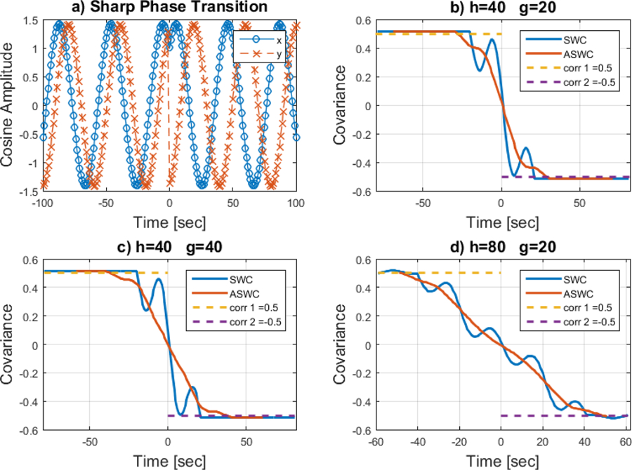
Figure 4. This plot shows a sharp correlation transition from 0.5 to −0.5.

a) The two cosines (f =0.025 Hz) suffer a phase change at time t=0 defining four different phases distributed among the two cosines. The phases were selected to simulate the configured correlations: cosine in blue shifted phase from π/4 to – π/4 radians, the red cosine from (π/4 – 0.5) to (− π/4 + 0.5) radians. b) Performing a tuned SWC with h = 40 sec shows the effect of the phase transition resulting in sinusoidal like artifacts. The effect of averaging g = 1/2f = 20 sec reduces the artifacts, but neither the phase transition nor the weighted averaging trend are removed as predicted in (7) and (8). C) In this plot we doubled the averaging length g =40 sec resulting in little change with respect to the original setup. d) Larger differences are observed when doubling the window length (h = 80 sec). As predicted in (8), changes in the window length will have a larger effect than changes in the averaging length.