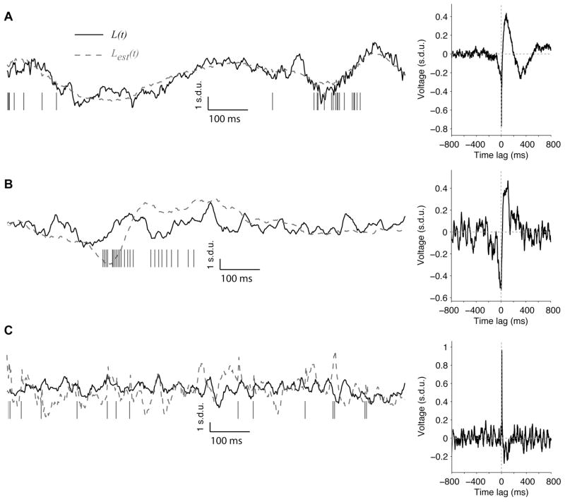
Figure 2. Examples of linear estimation of LFPs.
(A–C) Three examples of LFP estimations in 3 different electrodes recording V1 spontaneous activity. A random one-second sample is shown for each electrode; the firing rates and estimation accuracies are computed using a 240-second recording. The solid line shows the actual LFP and the dashed line shows the estimated LFP. The vertical ticks show the action potentials (MUA). On the right, we show the Wiener-Kolmogorov filter for each electrode (hmean). We only show the W-K filter for time lags between −800 ms and +800 ms; the number of points in the W-K filter was nfft+1 (nfft=2048). These examples illustrate the range of estimation levels that we observed (A: r=0.61, firing rate=46 Hz; B: r=0.29, firing rate=10 Hz; C: r=0.01, firing rate 13 Hz). More data segments for the electrode in 2A are shown in Figure S3B.

