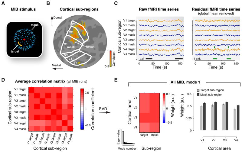
Figure 1. Correlation structure of cortical activity during MIB.
(A) Snapshot of the dynamic MIB stimulus. A salient yellow target was surrounded by a moving dot pattern (blue), which appeared as a rotating sphere. The target was presented in different visual field quadrants for different subjects. While viewing this stimulus, subjects repeatedly experienced and reported the spontaneous disappearance and reappearance of the target. (B) Cortical sub-regions. Separate localizer protocols delineated the sub-regions corresponding retinopically to the MIB target and the surrounding mask, within each of V1-V4 (highlighted for V1). The figure shows an example map of cortical responses to flickering probe stimulus presented at the spatial location of the MIB target. Colors represent correlation between measured activity and stimulus alternations (threshold: r > 0.5). The map is superimposed on a flattened representation of the subject’s occipital lobe. The borders of areas V1, V2, V3, and V4 are indicated as white outlines. The probe in the lower-left visual-field quadrant evoked responses in the dorsal sub-regions of right hemisphere visual areas V1-V3, and in the corresponding sub-region of area V4. (C) Example fMRI time series during one run of MIB. Left panel: “Raw” fMRI time series of the eight cortical sub-regions (yellow traces: target sub-regions; blue traces: mask sub-regions). The black bars at the bottom mark epochs of strong global fluctuations shared by all sub-regions. Right panel: Residual time series after removing the global mean across all sub-regions. The green bars and arrows mark epochs of anti-correlated fluctuations in the target and mask sub-regions of V4 (compare traces for target and mask subregions). Note the smaller scale than in the left panel. (D) Correlation matrix showing pair-wise correlation coefficients, for each pair of ROIs, averaged across all MIB runs and the six subjects. (E) Spatial mode, averaged across subjects. Left: Map of the spatial mode weights. The spatial modes are vectors, whose elements are re-organized as matrices (4 cortical areas × 2 subregions) for illustration. Right: Bar graph of the spatial mode weights. (Error bars: SEM, N=6) Inset: histogram of the eigenvalues. Gray bar, eigenvalue corresponding to the first spatial mode.

