
Figure 7. Comparison of average responses of real and model neurons.
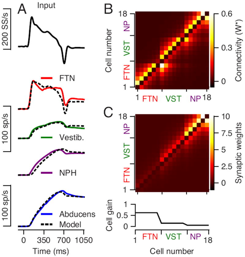
Dashed black and continuous curves illustrate the output from the model and the average firing rate of the data A: Continuous traces show average responses from our data and dashed traces show the output of an optimized model. From top to bottom the traces are: the input to model neurons #1-6 (FTNs), the average responses of FTNs, non-FTN vestibular neurons (model neurons #7-12), NPH neurons (model neurons #13-18), and Abducens neurons. We generated the activity of prepositus neurons according to their average sensitivity to eye kinematics in McFarland and Fuchs (1992). B: The colors show the effective connection strengths (W*) in the connection matrix between model neurons for a network that matches both temporal pattern and response amplitude. C: The colors in the image show the synaptic weights (referred to as Wsynapse in the Methods) and the graph at the bottom shows the internal gain of each model neuron. The gain values are: gFTN = 0.62; gVST = 0.14 gNPH = 0.05.