Figure 3.

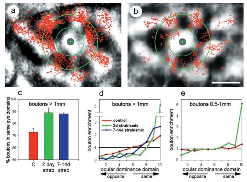
Ocular dominance distribution of anterogradely labeled boutons. a and b show the distribution of anterogradely labeled boutons (red) overlaid on optical maps of ocular dominance (grayscale background) for a normally sighted (a) and 2 d strabismic (b) kitten. The injection site in each case is marked by a gray circle enclosing a green +. The inner green circle marks a 500 μm radius from the injection site. The outer green circle marks a 1 mm radius from the injection site. Note that, in a, there are far more boutons present than in b, suggesting that a large fraction of the boutons may have been lost in this short time span. Scale bar (in b), 1 mm. A quantitative distribution of boutons relative to ocular dominance domains is shown in c and d for boutons that lie >1 mm from the injection site. As in Figure 2, control animals are shown in red, 2 d strabismic animals in green, and 7-14 d strabismic animals in blue. c graphs the percentage of boutons that lie within the half of the cortical area dominated by the eye that dominates the injection site. Error bars represent SEM. d plots the fraction of boutons per unit area in each of 10 ocular dominance zones. Colors are as in c, and ordinate and abscissa are as in Figure 2g. e plots this fraction for boutons lying between 500 μm and 1 mm from the injection site. Colors are as in c, and ordinate and abscissa are as in Figure 2g.