Brain Tumor Segmentation using Holistically-Nested Neural Networks in MRI Images

Abstract

Purpose

Gliomas are rapidly progressive, neurologically devastating, largely fatal brain tumors. Magnetic Resonance Imaging (MRI) is a widely used technique employed in the diagnosis and management of gliomas in clinical practice. MRI is also the standard imaging modality used to delineate the brain tumor target as part of treatment planning for the administration of radiation therapy. Despite more than 20 years of research and development, computational brain tumor segmentation in MRI images remains a challenging task. We are presenting a novel method of automatic image segmentation based on holistically-nested neural networks that could be employed for brain tumor segmentation of MRI images.

Methods

Two preprocessing techniques were applied to MRI images. The N4ITK method was employed for correction of bias field distortion. A novel landmark-based intensity normalization method was developed so that tissue types have a similar intensity scale in images of different subjects for the same MRI protocol. The holistically-nested neural networks (HNN), which extend from the convolutional neural networks (CNN) with a deep supervision through an additional weighted-fusion output layer, was trained to learn the multi-scale and multi-level hierarchical appearance representation of the brain tumor in MRI images and was subsequently applied to produce a prediction map of the brain tumor on test images. Finally, the brain tumor was obtained through an optimum thresholding on the prediction map.

Results

The proposed method was evaluated on both the Multimodal Brain Tumor Image Segmentation (BRATS) Benchmark 2013 training data sets, and clinical data from our institute. A dice similarity coefficient (DSC) and sensitivity of 0.78 and 0.81 were achieved on 20 BRATS 2013 training data sets with High Grade Gliomas (HGG), based on a two-fold cross-validation. The HNN model built on the BRATS 2013 training data was applied to 10 clinical data sets with HGG from a locally developed database. DSC and sensitivity of 0.83 and 0.85 were achieved. A quantitative comparison indicated that the proposed method outperforms the popular fully convolutional network (FCN) method. In terms of efficiency, the proposed method took around 10 hours for training with 50,000 iterations, and approximately 30 seconds for testing of a typical MRI image in the BRATS 2013 data set with a size of 160×216×176, using a DELL PRECISION workstation T7400, with an NVIDIA Tesla K20c GPU.

Conclusions

An effective brain tumor segmentation method for MRI images based on a HNN has been developed. The high level of accuracy and efficiency make this method practical in brain tumor segmentation. It may play a crucial role in both brain tumor diagnostic analysis and in the treatment planning of radiation therapy.

1. Introduction

Gliomas are rapidly progressive, neurologically devastating, largely fatal brain tumors.^{1, 2} Standard therapy consists of maximal surgical resection followed by observation for younger patients with tumors having good pathologic features and concurrent radiation therapy and temozolomide (TMZ) chemotherapy followed by adjuvant TMZ in high grade gliomas with poor prognostic features. In glioblastoma this approach results in an overall survival of 27.2% at 2 years and 9.8% at 5 years.³ Magnetic Resonance Imaging (MRI) is a widely used technique employed in the diagnosis, management and follow-up of gliomas in clinical practice. Radiation therapy treatment planning employs MRI as the standard imaging modality used to delineate the brain tumor target following co-registration with CT simulation images. Due to the high variation of brain tumor shape, size, and location, and particularly to the subtle intensity changes of tumor regions relative to the surrounding normal tissue, computational brain tumor segmentation in MRI is still a challenging task, in spite of more than 20 years of research and development.^{1, 4} Compounding this is the understanding of the infiltrative nature of gliomas that precludes the accurate identification of subclinical disease.^{5, 6} Currently, in most clinical radiotherapy treatment planning systems, manual contouring is the de facto standard for tumor delineation. It requires an operator with considerable skill and expertise in both tumor diagnostics and in the handling of the specific treatment planning software. Consequently, manual contouring is both time-consuming, and subject to large inter- and intra-observer variability. Semi- or fully-automatic brain tumor segmentation methods could circumvent this variability in radiotherapy treatment planning and could allow for the inclusion of advanced imaging techniques that are more challenging to human interpretation, e.g. diffusion weighted imaging, attenuated diffusion coefficient maps, magnetic resonance spectroscopy etc. Comprehensive reviews of existing brain tumor segmentation methods are provided by Mentz et al¹ and Bauer et al.² Mentz et al classified brain tumor segmentation methods into generative probabilistic based and discriminative approaches. Instead, we divided most brain tumor segmentation methods into semi- and fully-automatic groups.

For semi-automatic brain tumor segmentation, Guo, Schwartz and Zhao presented a method using active contours,⁷ where an approximate region of interest surrounding the tumor mass is initially manually contoured, after which a combination of global and local active contour models are utilized to segment the hyper-intense tumor. Raviv et al developed a latent atlas based approach for image ensembles segmentation.^{8, 9} A manual segmentation is required to initialize level-set propagation. Hamamci and Unal reported a method called “tumor-cut”,¹⁰ which combines the cellular automata based segmentation with graph-oriented methods. A maximum diameter of the tumor needs to be drawn by an expert to initialize segmentation. The basic set operations are utilized to combine the segmented volumes from different modalities. Moonis et al applied the fuzzy connectedness approach for tumor volume estimation, where seed points for brain tumors need to be specified by the user.¹¹ Njeh et al presented a graph cut distribution matching approach for glioma and edema segmentation in 3D multimodal MRI images.¹²

MRI based fully automatic brain tumor segmentation falls into several categories, including Bayesian and Markov random field (MRF),^{13, 14} atlas-based registration and combination of segmentation with registration,^15-17 statistical model of deformation,¹⁸ and support vector machine,^{19, 20} respectively. Recently, random forests (RF)^{21, 22} and convolutional neural networks (CNN)^{23, 24} have drawn more interest. Some researchers have successfully applied these two groups of algorithms to brain tumor segmentation for MRI images.^{4, 22, 25-30} Random forests represent machine learning algorithms that allow for the tumor classification. Many decision trees are constructed during training, and a class is assigned that claims the most votes of the individual trees during testing. The strength of the RF methods includes both its capability to naturally handle multiple-class of classifications and its characteristics utilizing large number of different features as the input vector. Tustison et al ²² employed RF for supervised tumor segmentation based on the feature sets of intensity, geometry, and asymmetry in multiple modality MRI images. The probability maps are initially generated from random forest models and are then used as spatial priors for a refining probabilistic segmentation based on Markov random field regularization. That algorithmic framework outperformed other methods in the Multimodal Brain Tumor Segmentation (BRATS) Benchmark challenge in the conference of MICCAI 2013.¹ Unlike RF approaches, which need variable specific features for classification, CNN-based methods have shown the advantages with respect to learning the hierarchy of complex features from in-domain data automatically³¹. They are usually used in image recognition systems,²⁴ but also recently in medical image analysis. CNN-based methods have shown effectiveness in mitosis detection in breast histologic images,³² and automatic pancreas segmentation in CT images,^{33, 34} and CT-based lymph node detection,³⁵ etc. For brain tumor segmentation, numerous CNN-based methods have been presented in both the MICCAI BRATS 2014 challenge ^{28, 36, 37} and BRATS 2015 challenge.^{4, 27, 38} Pereira et al ⁴ investigated using small 3×3 kernels to obtain deeper CNN, with data augmentation for brain tumor segmentation. Havaei et al³⁹ investigated several different CNN architectures for brain tumor segmentation, which employ the most recent advances in CNN design and training techniques, like Dropout regularization and Maxout hidden units, and also incorporate the local shape of tumors as well as their context. Zhao and Jia²⁶ designed multi-scale CNN for brain tumor segmentation and diagnosis, where both local and global features are incorporated in the image segmentation tasks.

Even though CNN-based methods demonstrate a promising performance in brain tumor segmentation, there is still room for improvement. Traditional standard CNN-based methods are typically patch-based for both training and testing. They predict the class of a pixel by processing an M×M (e.g. 32×32) square patch centered on that pixel and mainly focus on local features. In addition, in order to achieve a satisfactory class prediction, CNN methods typically require data augmentation to generate the large number of patches as additional training sets. In this paper, we investigate the use of holistically-nested neural networks (HNN) ⁴⁰ for brain tumor segmentation. The HNN was initially developed for edge detection using deep CNNs. However, it has also been shown to be effective in image object segmentation^{33, 35}. The HNN method has two advantages over traditional CNN: (1) holistic image training and prediction in an image-to-image fashion, rather than patch-based, where each pixel has a cost function; (2) multi-scale and multi-level image feature learning based on fully convolutional neural networks and deeply supervised nets. Hence, it is not necessary for the HNN to have a significant number of training data sets. Note that currently, the HNN is used for single object segmentation, in this paper we focus on enhanced brain tumor segmentation only.

The other contribution included in this paper is landmark-based image intensity normalization for MRI images. As mentioned in the references^{1, 4, 41}, MRI image intensity normalization plays a critical role in MRI image segmentation. In the patch-based CNN method for brain tumor segmentation, Unlike CT images, where pixel intensity is correlated to electron density, MRI image intensity doesn't have a tissue-specific physical meaning and can vary, for different image sets obtained with the same MRI protocol, from same/different scanners, and from same/different imaging centers. Most methods in the MICCAI BRATS challenges in 2013, 2014 and 2015 employed the histogram matching method ⁴² for MRI image intensity normalization. Histogram matching strongly depends on the histogram shape. In some cases, this method may not work well, due to the large variability of the brain tumor in size as well as in pixel intensities that may cause a different shape of the histogram. In this paper, a novel method for image intensity normalization was developed that is simple and effective. The white matter corresponding to the highest histogram bin was chosen as the landmark. Segment linear transformation was then performed to map this landmark to the standard intensity normalization scale.

2. Materials and Methods

2.A. Data

Twenty high grade glioma (HGG) data sets from the BRATS 2013 training data were utilized for training and testing. These data were generated on a variety of scanners with different field strengths. Testing data also include 10 clinical data sets with HGG from a locally developed database. Each data set was comprised of four MRI modalities: T1-weighted (T1), contrast enhanced T1-weighted (T1c), T2-weighted and T2-FLAIR images to provide complimentary biological information. All images were co-registered to the same anatomical reference using a rigid transform with a mutual information similarity metric implemented in ITK.⁴³ All images were skull-stripped and interpolated to 1×1×1mm³ voxel resolution.

2.B. Image Preprocessing

In MRI image analysis, there are two common artifacts that can affect the performance of image processing algorithms. These are (1) the bias field distortion and (2) the non-physical meaning of the MRI image intensities. The first shows a slowly-varying, inhomogeneous background in an MRI image. This correction of bias field distortion has been addressed extensively and many effective methods have been developed.^{44, 45} The latter artifact implies the lack of a tissue-specific numeric meaning of the MRI pixel intensities. The importance of handling such MRI intensity normalization has been emphasized the literature.^{4, 41, 42} In the first step of our image preprocessing, the bias field distortion in MRI images were corrected using the well-known N4ITK method.⁴⁵ Then, the intensity of each MRI image was normalized using a novel, landmark-based method we have developed, to make the histogram of MRI images of each modality more similar across different subjects. In this paper, the landmark is chosen as the intensity value associated with the highest histogram bin of each image (ignoring the black background), which typically corresponds to the white matter tissue since it occupies the largest volume of the brain. The MRI image and the corresponding histogram of each MRI protocol are shown in Figure 1.

Figure 1.

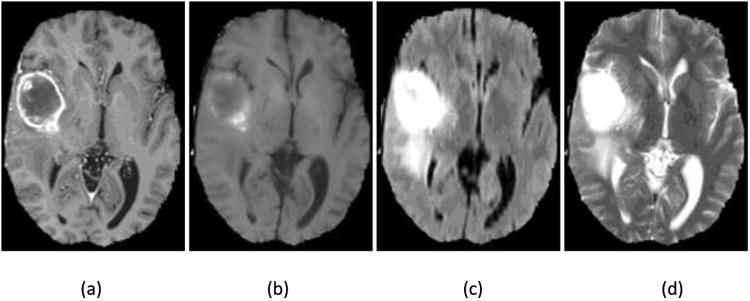
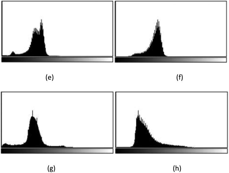
One slice of MRI images with different sequences from the BRATS 2013 one HGG patient data. (a) T1 contrast enhanced image, (b) T1-weighted image, (c) T2 Flair image, (d) T2-weighted image; Corresponding histograms (e)obtained from T1c, (f) from T1, (g) from T2 Flair, and (h) from T2.

Once the landmark is generated for each MRI image, a piecewise linear transform is performed by mapping the landmark intensity to the normalized intensity scale, as illustrated in Figure 2. Here, the segment linear transformation is chosen due to its simplicity and effectiveness in producing similar histograms of MRI images across different subjects. As mentioned in the original intensity normalization paper,⁴² other transformation like using polynomial functions or split fitting techniques to stretch histogram segments may also be used, but it is out of the scope of the paper. The abscissa represents the intensities in a test image where the landmark has intensity value I_m, and the ordinate denotes the normalized reference intensities. Additionally, I₁ is taken to be the smallest intensity over the test image and I₂ to be the intensity at the 99.9^th percentile within the test image. Beyond 99.9 percent, the intensities represent mostly outlier values. The landmarks of I_m obtained from the histogram of each image of a subset of images are mapped to the normalized reference intensity scale by linearly mapping the intensities from [I₁, I₂] to [r₁, r₂] (e.g. [0,4095]), in such a way, the map I′_m of I_m on [r₁, r₂] can be obtained. The landmark intensity r_m on the reference scale is then determined and fixed as the rounded mean of the I′_ms. For any test image, once parameters of I₁, I₂ and I_m are obtained, two corresponding slopes of the piecewise linear transformation are calculated since parameters of r₁, r₂ and r_m on the reference scale are fixed.

Figure 2.

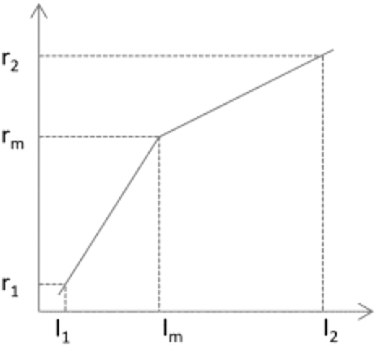
Illustration of the landmark-based MRI intensity normalization.

2.C. Holistically-Nested Neural Networks (HNN)

Unlike traditional CNNs, which perform a pixel classification prediction using patch-based approaches, as shown in Figure 3(a), and make use of the local correlation between the intensities of that pixel and adjacent pixels, the HNN-based method performs learning and prediction in an image-to-image fashion, by combining multi-scale and multi-level hierarchical intensity representations of the image. HNN is an extension of traditional CNNs and is able to produce predictions from multiple scales. The HNN architecture comprises a single-stream deep network with multiple side outputs, as shown in Figure 3(b), and each corresponds to one image scale. Each side output is associated with one side-output layer, which has a separate classifier. An additional weighted-fusion layer is added to the HNN architecture to unify the multiple side outputs. The fusion weight parameters are learned simultaneously in the training step. In this paper, a holistic image segmentation method employing the holistically-nested neural networks⁴⁰ was present for brain tumor segmentation in MRI images, wherein both training and testing take 2D MRI image slices as input. The HNN was initially developed for edge detection using deep CNNs. It has also been demonstrated that it is also effective in image object segmentation^33-35. The paper follows the same notation as utilized in the HNN reference paper ^{34, 40}.

Figure 3.

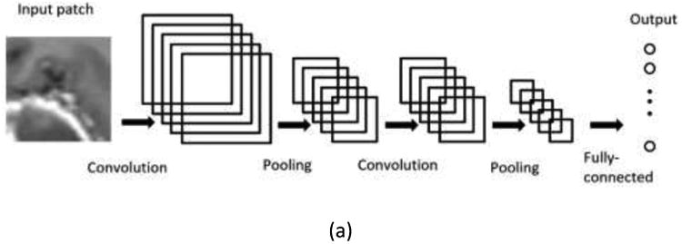
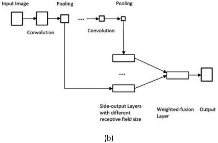
Illustration of neural network architectures: (a) Traditional CNN architecture; (b) HNN architecture.

The HNN formulation: The training data is denoted as S = {(X_n, Y_n), n = 1, …, N}, where X_n denotes the input MRI image consisting of four MRI protocols, as previously mentioned in Section 2.A., and $Y_n=\{y_j^{(n)},j=1,\cdots ,|X_n|\}$, $y_j^{(n)}\in \{0,1\}$ denotes the corresponding ground truth of the brain tumor for image X_n. In the training data, positive samples represent pixels of brain tumor and negative samples represent non-tumor pixels. Suppose the collection of all standard CNNs network layer parameters is denoted as W, and we have K side-output layers with the corresponding weights denoted by w = (w⁽¹⁾,…, w^(K)). We then define the objective function as

$$L_{\mathit{\text{side}}}(W,w)=\sum _{k=1}^K{\alpha }_k{l}_{\mathit{\text{side}}}^{(k)}(W,w^{(k)}),$$

where $l_{\mathit{\text{side}}}^{(k)}$ denotes the image-level loss function for the k^th side-output. In the image-to-image fashion training, the loss function is computed over all pixels in a training image X_n and corresponding ground truth Y_n. There is a heavy bias towards non-tumor pixels in a typical MRI image with brain tumor. Therefore, to balance the loss between object and non-object classes, an additional trade-off parameter β is introduced by Xie and Tu.⁴⁰ Thus, a class-balanced cross-entropy loss function can be used in the above objective function:

$$l_{\mathit{\text{side}}}^{(k)}(W,w^{(k)})=-\beta \sum _{j\in Y_{+}}logPr(y_j=1|X;W,w^{(k)})-(1-\beta )\sum _{j\in Y_{+}}logPr(y_j=0|X;W,w^{(k)})$$

where β = |Y₋|/|Y| and 1 – β = |Y₊|/|Y|. |Y₋|and |Y₊| denote the ground truth set of negative and positive samples, respectively. $Pr(y_i=1|X;W,w^{(k)})=\sigma (a_j^{(k)})\in [0,1]$ is computed on the activation value at each pixel j using the sigmoid function σ(.). At each side-output layer, a single object prediction map ${\widehat{Y}}_{\mathit{\text{side}}}^{(k)}=\sigma \left({\widehat{A}}_{\mathit{\text{side}}}^{(k)}\right)$ is produced, where ${\widehat{A}}_{\mathit{\text{side}}}^{(k)}\equiv \{a_j^{(k)}j=1,\cdots ,|Y|\}$ are activations of the side-output of layer k. An additional weighted-fusion layer is then added to the network architecture to combine side-output predictions. The fusion weights are learned simultaneously during the training step. The final loss function at the fusion layer is defined as

$$L_{\mathit{\text{fuse}}}(W,w,h)=\mathit{\text{Dist}}(Y,{\widehat{Y}}_{\mathit{\text{fuse}}}),$$

where ${\widehat{Y}}_{\mathit{\text{fuse}}}\equiv \sigma \left({\sum }_{k=1}^K{h}_k{\widehat{A}}_{\mathit{\text{side}}}^{(k)}\right)$ with h = (h₁, …, h_K) being the fusion weights. Dist(Y,Ŷ_fuse) represents the distance between the fused predictions Ŷ_fuse and the ground truth label map Y, which is set to be a cross-entropy loss. Finally, the overall objective function can be minimized by using the stochastic gradient descent approach:

$$(W,w,h)\ast =argmin(L_{\mathit{\text{side}}}(W,w)+L_{\mathit{\text{fuse}}}(W,w,h))$$

In testing, for any given image X, tumor map predictions from both the weighted-fusion layer and the side output layers are obtained: $({\widehat{Y}}_{\mathit{\text{fuse}}},{\widehat{Y}}_{\mathit{\text{side}}}^{(1)},\cdots ,{\widehat{Y}}_{\mathit{\text{side}}}^{(K)})=\mathit{\text{HNN}}(X,(W,w,h)\ast )$, where HNN(·) denotes the object maps produced by the network. The final unified output is then produced by a further weighted averaging of all these generated prediction maps. ${\widehat{Y}}_{\mathit{\text{HED}}}=\mathit{\text{Average}}({\widehat{Y}}_{\mathit{\text{fuse}}},{\widehat{Y}}_{\mathit{\text{side}}}^{(1)},\cdots ,{\widehat{Y}}_{\mathit{\text{side}}}^{(K)})$. In this work, we take the Ŷ_fuse as the final prediction map. An example is shown in Figure 4.

Figure 4.

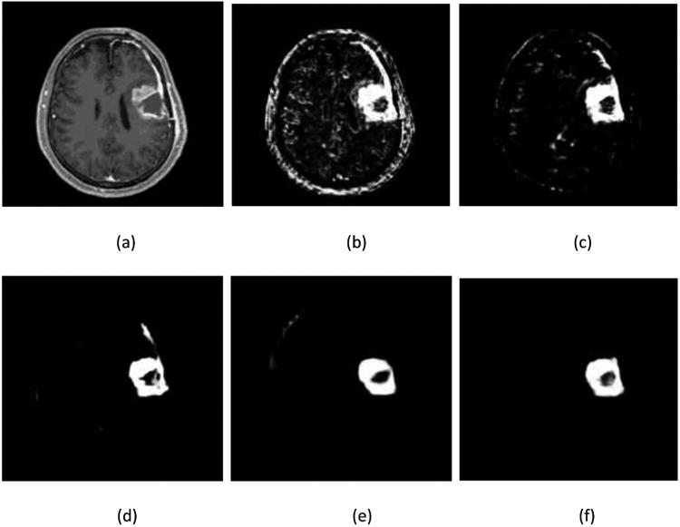
Illustration of output prediction maps. (a) one slice of the T1c component of input MRI image; and corresponding prediction maps (b) from the first side-output layer;(c) from the second side-output layer; (e) from the third side-output layer; (e) from the 4^th side-output layer; (f) from the fusion layer.

2.D. Post-processing

To produce binary segmentation results from the prediction map, a simple thresholding technique is applied. The optimal threshold value is set to maximize the mean DSC between the binary segmentation and the ground truth of the two training folds. Small connected-components that are below a certain volume are discarded.

3. Results

In this section, the performance of the proposed HNNs-based approach for brain tumor segmentation in MRI images was evaluated. As we mentioned earlier, the focused was on the enhanced tumor segmentation in this work, since the HNN is currently developed for single object segmentation, and is not able to classify the whole tumor region into four classes: necrosis, edema, non-enhancing tumor, and enhancing tumor. The evaluation was performed on the 20 data from the BRATS 2013 training data sets using two-fold cross validation. These 20 HGG data are divided into two folds, each one contains 10 cases. Segmentation results are produced on one fold by the HNN which was then trained on the other fold. Manual enhanced tumor delineations by anonymous human experts were taken as ground truths.¹ Metrics of dice similarity coefficient (DSC) ⁴⁶ and sensitivity were then calculated. DSC is commonly utilized to measure the similarity between results from manual and automatic segmentation methods, and is defined as

$$\text{DSC}(\mathrm{A},\mathrm{B})=\frac{2(|A\cap B|)}{(|A|+|B|)},$$

where A represents the result from automatic segmentation method and B represents the result from manual segmentation, and |A|denotes the number of voxels in image A with value 1. The DSC value is 1 when the two segmentation results are identical and 0 when they are completely disjoint.

Sensitivity is usually used to measure fraction of positives that are correctly identified by a certain segmentation method. It is defined as

$$\text{Sensitivity}=\frac{\mathit{\text{TP}}}{\mathit{\text{TP}}+\mathit{\text{FN}}},$$

where TP represents the number of true positive and FN is the number of false negative. Measurements from the proposed method were compared with the popular fully convolutional networks (FCN) method.^{47, 48} The results of comparison are shown in Table 1. It is shown that the HNN-based method outperformed the FCN method, on the BRATS 2013 training data sets. Note that the FCN implementation we adopted is based on the FCN-8s network, which is publicly available at http://fcn.berkeleyvision.org. The data fed into the FCN method are those after two-step preprocessing as described in Section 2.B.

Table 1.

Performance comparison of enhancing tumor segmentation between the proposed HNN-based method, and the FCN method, on the high-grade training data from the BRATS 2013.

Method	DSC	Sensitivity
FCN	0.61	0.65
Proposed HNN-based	0.78	0.81

In Figure 5, an example of the segmentation of one HGG patient from BRATS 2013 data sets is presented.

Figure 5.

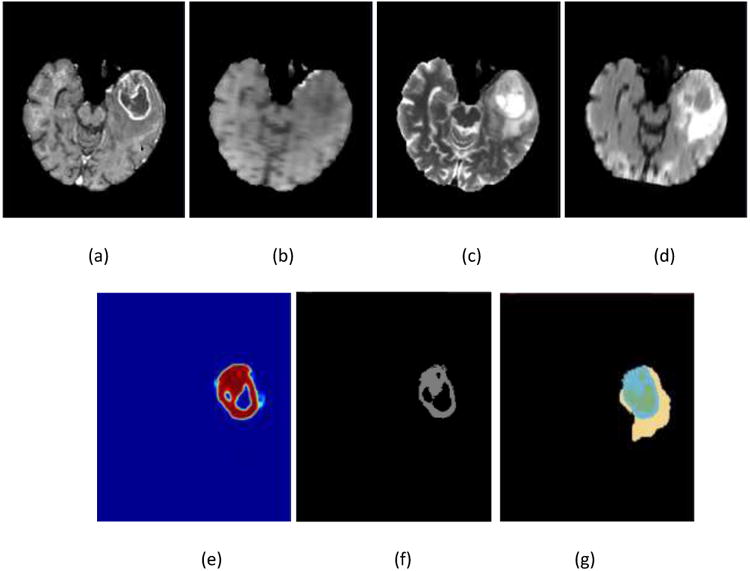
Illustration of the enhanced tumor segmentation using our proposed HNN method on one HGG patient from BRATS 2013 data sets. The four images in the first row shows the MRI modalities. (a) T1c, (b) T1, (c) T2, (d) Flair. Images in the bottom row from left to right are (e) prediction map, (f) final binary segmentation after optimal thresholding on prediction map, and (g) ground truth where light blue color represents enhanced tumor.

In addition, the proposed method was used to evaluate clinical data where the HNN was trained using the same BRATS 2013 training data. Ten patient data sets were randomly chosen with HGG from a locally developed database. Like BRATS data sets, each patient data set consisted of four modalities: T1c, T1, T2, and Flair weighted images. Figure 6 shows an example, and Table 2 lists the measurements of DSC and sensitivity of the proposed HNN-based method, and comparison with the FCN method. Note Ground truths in the performance evaluation were manually contoured by a clinical radiation oncologist.

Figure 6.

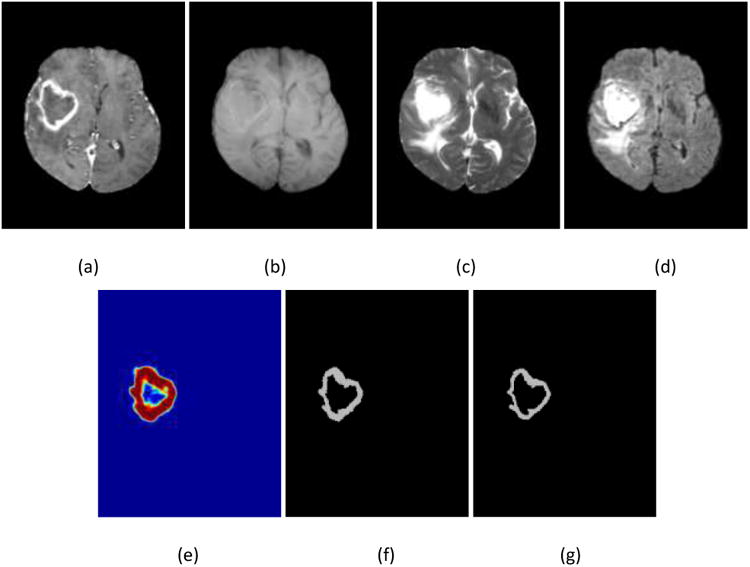
Illustration of the enhanced tumor segmentation using proposed HNN method on clinical data from a local database where the HNN is trained on BRATS 2013 data sets. (a) T1c, (b) T1, (c) T2, (d) Flair, (e) prediction map, (f) binary segmentation, and (g) ground truth.

Table 2.

Performance evaluation of the proposed HNN-based method, and comparison with the FCN method on 10 clinical data sets with HGG from a local database.

Method	DSC	Sensitivity
FCN	0.67	0.70
Proposed HNN-based	0.83	0.85

According to the results shown in Table 2, both DSC and Sensitivity of the proposed HNN method and the FCN method, on 10 patient sets with HGG from a clinical database were improved relative to those of the BRATS 2013 data sets. One reason might be the difference of image quality between two data sets. The other reason could be the difference in the ground truth. Different observers have different preferences in manually contouring ground truth and these sometimes show significant variances, even on same data sets. The proposed HNN method outperformed the FCN method in terms of both the DSC and sensitivity.

The proposed HNN-based method is implemented based on the HED system⁴⁰ using the publicly available Caffe platform⁴⁹, and is executed on a DELL WORKSTATION T7400 with a quad-core 2.66 GHZ Xeon CPU, with 32 GB memory under the CentOS 6.6 Linux operating system. A GPU NVIDIA Tesla K20c with 5 GB device memory was used. The program takes around 10 hours for training with 50000 iterations, and takes only around 30 seconds for testing of a typical image set with a size of 160×216×176. In efficiency, the proposed HNN-based method outperforms most CNN-based methods. ^{1, 4, 36, 37} Pereira reports an average running time of 8 min for one BRATS 2013 data,⁴ on an Intel Core i7 3.5 GHz machine, using a GPU NVIDIA GeForce GTX 980. The difference in running times may be due to the processing of substantial number of patches in their method. In addition, their method adopted a different network architecture, which has more deeper layers while the proposed method only has 5 stages with a trimmed VGGNet network.

4. Discussion

The entire network of the HNN method is fine-tuned from initialization based on a pre-trained model VGGNet on ImageNet.⁵⁰ In this manner, multi-scale and multi-level image features can be efficiently generated due to the deep architecture derived from the VGGNet. Unlike the traditional CNN networks where data augmentation is a common procedure to improve prediction accuracy^{4, 39}, the HNN doesn't require a large number of training data sets. In our experiments, the HNN model was trained on 10 data from the BRATS 2013 data sets and can be effectively applied to segmentation on clinical data sets.

We followed the implementation of the original HED system.⁴⁰ The final network architecture has 5 stages, with strides of 1, 2, 4, 8, and 16, respectively, all nested in the trimmed VGGNet. In each stage, the final convolutional layer is connected to one side output layer with corresponding receptive field size. In addition, the same hyper-parameters as the HED system are used, which include the learning rate of 1e-6, momentum of 0.9, the loss-weight α_k of 1 for each side-output layer. The final fusion layer weights after network training convergence are h = (0.19967, 0.20004, 0.20070, 0.20059, 0.20078).

As for the image intensity normalization, in our implementation, we mapped the intensity scale of a given test MRI image to intensity range from 0 to 4095 via a piecewise linear transformation, in such a way there is less information loss during intensity normalization. The slices of a three-dimensional MRI image were saved as a series of JPEG files with intensity scaled to range between 0 and 255. These JPEG files were finally fed into the Caffe platform. Pereira et al ⁴ reported that the metrics of DSC and sensitivity from the method (patch-based CNN) had obtained a mean gain of 4.6% by pre-processing using Nyul's intensity normalization.⁴² It is shown that in MRI application, CNN-based classifiers improved performance after intensity normalization. The performance difference of the proposed HNN-based method (image-to-image fashion, multi-scale CNN) before and after intensity normalization will be further investigated in the future.

5. Conclusions

In this paper, a novel automatic brain tumor segmentation method based on holistically-nested neural networks (HNN) has been described. Two preprocessing techniques, namely Bias Field Inhomogeneity Correction and Intensity Normalization, were first applied to MRI images. Multi-scale and multi-level hierarchical image features were learned through the HNN training. Unlike the traditional CNN methods which are patch-based and mainly focus local features, the HNN method performed both training and prediction based on holistic image-to-image fashion.

The performance of the proposed HNN method was evaluated on 20 HGG BRATS 2013 training data sets and 10 patient data sets with HGG from a clinical database. A dice similarity coefficient and sensitivity of 0.78 and 0.81 for the BRATS 2013 data, 0.83 and 0.85 for clinical data have been achieved, respectively. Thanks to the landmark-based intensity normalization technique, the HNN training model can also be effectively utilized for testing clinical HGG data. The proposed method outperformed the FCN method based on a quantitative comparison. Note that the dice coefficient and sensitivity of the enhanced tumor segmentation produced by the state-of-the-art CNN methods are 0.73 and 0.80,³⁹ and 0.77 and 0.81,⁴ respectively, on the BRATS 2013 Challenge data. Unfortunately, the HNN-based method focused only on single object segmentation, and doesn't have access an online evaluation system. We are extending the HNN-based method from single object segmentation to simultaneous multiple-object segmentation. In the future, the application of the HNN-based method on the Challenge data will be investigated so that a comprehensive comparison with the state-of-the-art CNN methods can be performed. Other applications of the HNN-based method like organ-at-risk in head and neck images will also be investigated. In efficiency, the HNN method is built on top of the HED system,⁴⁰ due to the efficient implementations of both the Caffe platform⁴⁹ and the HED system,⁴⁰ this method takes approximately 30 seconds to segment the enhanced brain tumor in a reference data set. Both increased accuracy and efficiency make the HNN a very practical segmentation method which may play an important role in both diagnosis and radiation therapy treatment planning.

References

- 1.Menze BH, Jakab A, Bauer S, Kalpathy-Cramer J, Farahani K, Kirby J, Burren Y, Porz N, Slotboom J, Wiest R, Lanczi L, Gerstner E, Weber MA, Arbel T, Avants BB, Ayache N, Buendia P, Collins DL, Cordier N, Corso JJ, Criminisi A, Das T, Delingette H, Demiralp C, Durst CR, Dojat M, Doyle S, Festa J, Forbes F, Geremia E, Glocker B, Golland P, Guo X, Hamamci A, Iftekharuddin KM, Jena R, John NM, Konukoglu E, Lashkari D, Mariz JA, Meier R, Pereira S, Precup D, Price SJ, Raviv TR, Reza SM, Ryan M, Sarikaya D, Schwartz L, Shin HC, Shotton J, Silva CA, Sousa N, Subbanna NK, Szekely G, Taylor TJ, Thomas OM, Tustison NJ, Unal G, Vasseur F, Wintermark M, Ye DH, Zhao L, Zhao B, Zikic D, Prastawa M, Reyes M, Van Leemput K. The Multimodal Brain Tumor Image Segmentation Benchmark (BRATS) IEEE transactions on medical imaging. 2015;34:1993–2024. doi: 10.1109/TMI.2014.2377694. [DOI] [PMC free article] [PubMed] [Google Scholar]
- 2.Bauer S, Wiest R, Nolte LP, Reyes M. A survey of MRI-based medical image analysis for brain tumor studies. Physics in medicine and biology. 2013;58:R97–129. doi: 10.1088/0031-9155/58/13/R97. [DOI] [PubMed] [Google Scholar]
- 3.Stupp R, Hegi ME, Mason WP, van den Bent MJ, Taphoorn MJ, Janzer RC, Ludwin SK, Allgeier A, Fisher B, Belanger K, Hau P, Brandes AA, Gijtenbeek J, Marosi C, Vecht CJ, Mokhtari K, Wesseling P, Villa S, Eisenhauer E, Gorlia T, Weller M, Lacombe D, Cairncross JG, Mirimanoff RO. Effects of radiotherapy with concomitant and adjuvant temozolomide versus radiotherapy alone on survival in glioblastoma in a randomised phase III study: 5-year analysis of the EORTC-NCIC trial. The Lancet Oncology. 2009;10:459–466. doi: 10.1016/S1470-2045(09)70025-7. [DOI] [PubMed] [Google Scholar]
- 4.Pereira S, Pinto A, Alves V, Silva CA. Brain Tumor Segmentation Using Convolutional Neural Networks in MRI Images. IEEE Transaction on Medical Imaging. 2016;35:1240–1251. doi: 10.1109/TMI.2016.2538465. [DOI] [PubMed] [Google Scholar]
- 5.Burger PC, Vogel FS, Green SB, Strike TA. Glioblastoma multiforme and anaplastic astrocytoma. Pathologic criteria and prognostic implications. Cancer. 1985;56:1106–1111. doi: 10.1002/1097-0142(19850901)56:5<1106::aid-cncr2820560525>3.0.co;2-2. [DOI] [PubMed] [Google Scholar]
- 6.Sahm F, Capper D, Jeibmann A, Habel A, Paulus W, Troost D, von Deimling A. Addressing diffuse glioma as a systemic brain disease with single-cell analysis. Archives of Neurology. 2012:523–526. doi: 10.1001/archneurol.2011.2910. [DOI] [PubMed] [Google Scholar]
- 7.Guo XG, Schwartz L, Zhao B. Semi-automatic Segmentation of Multimodal Brain Tumor Using Active Contours. Medical Image Computing and Computer Assisted Intervention. 2013:27–30. [Google Scholar]
- 8.Raviv TR, Van Leemput K, Menze BH, Wells WM, 3rd, Golland P. Segmentation of image ensembles via latent atlases. Medical image analysis. 2010;14:654–665. doi: 10.1016/j.media.2010.05.004. [DOI] [PMC free article] [PubMed] [Google Scholar]
- 9.Raviv TR, Van Leemput K, Wells WM, 3rd, Golland P. Joint segmentation of image ensembles via latent atlases. Medical image computing and computer-assisted intervention :MICCAI … International Conference on Medical Image Computing and Computer-Assisted Intervention. 2009;12:272–280. doi: 10.1007/978-3-642-04268-3_34. [DOI] [PMC free article] [PubMed] [Google Scholar]
- 10.Hamamci A, Kucuk N, Karaman K, Engin K, Unal G. Tumor-Cut: segmentation of brain tumors on contrast enhanced MR images for radiosurgery applications. IEEE transactions on medical imaging. 2012;31:790–804. doi: 10.1109/TMI.2011.2181857. [DOI] [PubMed] [Google Scholar]
- 11.Moonis G, Liu J, Udupa JK, Hackney DB. Estimation of tumor volume with fuzzy-connectedness segmentation of MR images. AJNR American journal of neuroradiology. 2002;23:356–363. [PMC free article] [PubMed] [Google Scholar]
- 12.Njeh I, Sallemi L, Ayed IB, Chtourou K, Lehericy S, Galanaud D, Hamida AB. 3D multimodal MRI brain glioma tumor and edema segmentation: a graph cut distribution matching approach. Computerized Medical Imaging and Graphics. 2015;40:108–119. doi: 10.1016/j.compmedimag.2014.10.009. [DOI] [PubMed] [Google Scholar]
- 13.Prastawa M, Bullitt E, Ho S, Gerig G. A brain tumor segmentation framework based on outlier detection. Medical image analysis. 2004;8:275–283. doi: 10.1016/j.media.2004.06.007. [DOI] [PubMed] [Google Scholar]
- 14.Bauer S, Seiler C, Bardyn T, Buechler P, Reyes M. Atlas-based segmentation of brain tumor images using a Markov random field-based tumor growth model and non-rigid registration. Conference proceedings : … Annual International Conference of the IEEE Engineering in Medicine and Biology Society IEEE Engineering in Medicine and Biology Society Annual Conference. 2010;2010:4080–4083. doi: 10.1109/IEMBS.2010.5627302. [DOI] [PubMed] [Google Scholar]
- 15.Prastawa M, Bullitt E, Moon N, Van Leemput K, Gerig G. Automatic brain tumor segmentation by subject specific modification of atlas priors. Academic radiology. 2003;10:1341–1348. doi: 10.1016/s1076-6332(03)00506-3. [DOI] [PMC free article] [PubMed] [Google Scholar]
- 16.Cuadra MB, Pollo C, Bardera A, Cuisenaire O, Villemure JG, Thiran JP. Atlas-based segmentation of pathological MR brain images using a model of lesion growth. IEEE transactions on medical imaging. 2004;23:1301–1314. doi: 10.1109/TMI.2004.834618. [DOI] [PubMed] [Google Scholar]
- 17.Kwon D, Shinohara RT, Akbari H, Davatzikos C. Combining Generative Models for Multifocal Glioma Segmentation and Registration. Medical image computing and computer-assisted intervention : MICCAI … International Conference on Medical Image Computing and Computer-Assisted Intervention. 2014:763–770. doi: 10.1007/978-3-319-10404-1_95. [DOI] [PMC free article] [PubMed] [Google Scholar]
- 18.Mohamed A, Zacharaki EI, Shen D, Davatzikos C. Deformable registration of brain tumor images via a statistical model of tumor-induced deformation. Medical image analysis. 2006;10:752–763. doi: 10.1016/j.media.2006.06.005. [DOI] [PubMed] [Google Scholar]
- 19.Bauer S, Nolte Lp, Reyes M. Fully automatic segmentation of brain tumor images using support vector machine classification in combination with hierarchical conditional random field regularization. Medical image computing and computer-assisted intervention :MICCAI … International Conference on Medical Image Computing and Computer-Assisted Intervention. 2011:354–361. doi: 10.1007/978-3-642-23626-6_44. [DOI] [PubMed] [Google Scholar]
- 20.Zhang N, Ruan S, Lebonvallet S, Liao Q, Zhu Y. Kernel feature selection to fuse multi-spectral MRI images for brain tumor segmentation. Computer Vision and Image Understanding. 2011;115:256–259. [Google Scholar]
- 21.Breiman L. Random forests. Machine Learning. 2001;45:5–32. [Google Scholar]
- 22.Tustison NJ, Shrinidhi KL, Wintermark M, Durst CR, Kandel BM, Gee JC, Grossman MC, Avants BB. Optimal Symmetric Multimodal Templates and Concatenated Random Forests for Supervised Brain Tumor Segmentation (Simplified) with ANTsR. Neuroinformatics. 2015;13:209–225. doi: 10.1007/s12021-014-9245-2. [DOI] [PubMed] [Google Scholar]
- 23.LeCun Y, Bengio Y, Hinton G. Deep learning. Nature. 2015;521:436–444. doi: 10.1038/nature14539. [DOI] [PubMed] [Google Scholar]
- 24.Krizhevsky A, Sutskever I, Hinton GE. ImageNet Classification with Deep Convolutional Neural Networks. Advances in Neural Information Processing Systems. 2012;1:1097–1115. [Google Scholar]
- 25.Meier R, Bauer S, Slotboom J, Wiest R, Reyes M. Appearance- and context-sensitive features for brain tumor segmentation. Medical image computing and computer-assisted intervention : MICCAI … International Conference on Medical Image Computing and Computer-Assisted Intervention. 2014:20–26. doi: 10.1007/978-3-319-10404-1_89. [DOI] [PubMed] [Google Scholar]
- 26.Zhao L, Jia K. Multiscale CNNs for Brain Tumor Segmentation and Diagnosis. Computational and Mathematical Methods in Medicine. 2016;2016:8356291–8356297. doi: 10.1155/2016/8356294. 8356294. [DOI] [PMC free article] [PubMed] [Google Scholar]
- 27.Havaei M, Dutil F, Pal C, Larochelle H, Jodoin PM. A Convolutional Neural Network Approach to Brain Tumor Segmentation. MICCAI Multimodal Brain Tumor Segmentation Challenge (BraTS) 2015:29–33. [Google Scholar]
- 28.Zikic D, Ioannou Y, Brown M, Criminisi A. Segmentation of Brain Tumor Tissues with Convolutional Neural Networks. MICCAI Multimodal Brain Tumor Segmentation Challenge (BraTS) 2014:36–39. [Google Scholar]
- 29.Maier O, Wilms M, Handels H. Highly disciminative features for Glima Segmentation in MR Volumes with Random Forests. MICCAI Multimodal Brain Tumor Segmentation Challenge (BraTS) 2015:38–41. [Google Scholar]
- 30.Pinto A, Pereira S, Correia H, Oliveira J, Rasteiro DM, Silva CA. Brain Tumour Segmentation based on Extremely Randomized Forest with high-level features. Conf Proc IEEE Eng MedBiol Soc. 2015:3037–3040. doi: 10.1109/EMBC.2015.7319032. [DOI] [PubMed] [Google Scholar]
- 31.Bengio Y, Courville A, Vincent P. Representation Learning: A Review and New Perspectives. IEEE Trans Pattern Anal Mach Intell. 2013;35:1798–1828. doi: 10.1109/TPAMI.2013.50. [DOI] [PubMed] [Google Scholar]
- 32.Cireşan DC, Giusti A, Gambardella LM, Schmidhuber J. Mitosis Detection in Breast Cancer Histology Images with Deep Neural Networks. In: Mori K, Sakuma I, Sato Y, Barillot C, Navab N, editors. Proceedings, Part II; Medical Image Computing and Computer-Assisted Intervention – MICCAI 2013: 16th International Conference; Nagoya, Japan. September 22-26, 2013; Berlin, Heidelberg: Springer Berlin Heidelberg; 2013. pp. 411–418. [DOI] [PubMed] [Google Scholar]
- 33.Roth HR, Lu L, Farag A, Shin HC, Liu J, Turkbey EB, Summers RM. Deep Organ: Multi-level Deep Convolutional Networks for Automated Pancreas Segmentation. In: Navab N, Hornegger J, Wells MW, Frangi FA, editors. Proceedings, Part I; Medical Image Computing and Computer-Assisted Intervention -- MICCAI 2015: 18th International Conference; Munich, Germany. October 5-9, 2015; Cham: Springer International Publishing; 2015. pp. 556–564. [Google Scholar]
- 34.Roth HR, Lu L, Farag A, Sohn A, Summers RM. Spatial Aggregation of Holistically-Nested Networks for Automated Pancreas Segmentation. In: Ourselin S, Joskowicz L, Sabuncu MR, Unal G, Wells W, editors. Proceedings, Part II; Medical Image Computing and Computer-Assisted Intervention – MICCAI 2016: 19th International Conference; Athens, Greece. October 17-21, 2016; Cham: Springer International Publishing; 2016. pp. 451–459. [Google Scholar]
- 35.Roth HR, Lu L, Seff A, Cherry KM, Hoffman J, Wang S, Liu J, Turkbey E, Summers RM. ANew 2.5D Representation for Lymph Node Detection Using Random Sets of Deep Convolutional Neural Network Observations. In: Golland P, Hata N, Barillot C, Hornegger J, Howe R, editors. Proceedings, Part I; Medical Image Computing and Computer-Assisted Intervention – MICCAI 2014: 17th International Conference; Boston, MA, USA. September 14-18, 2014; Cham: Springer International Publishing; 2014. pp. 520–527. [DOI] [PMC free article] [PubMed] [Google Scholar]
- 36.Urban G, Bendszus M, Hamprecht F, Kleesiek J. Multi-modal Brain Tumor Segmentation using Deep Convolutional Neural Networks. MICCAI Multimodal Brain Tumor Segmentation Challenge (BraTS) 2014:1–5. [Google Scholar]
- 37.Davy A, Havaei M, Warde-farley D\, Biard A, Tran L, Courville A, Larochelle H, Pal C, Bengio Y. Brain Tumor Segmentation with Deep Neural Networks. MICCAI Multimodal Brain Tumor Segmentation Challenge (BraTS) 2014:1–5. [Google Scholar]
- 38.Rao V, Sarabi MS, Jaiswal A. Brain Tumor Segmentation with Deep Learning. MICCAI Multimodal Brain Tumor Segmentation Challenge (BraTS) 2015:56–59. [Google Scholar]
- 39.Havaei M, Davy A, Warde-Farley D, Biard A, Courville A, Bengio Y, Pal C, Jodoin PM, Larochelle H. Brain tumor segmentation with Deep Neural Networks. Medical image analysis. 2017;35:18–31. doi: 10.1016/j.media.2016.05.004. [DOI] [PubMed] [Google Scholar]
- 40.Xie S, Tu Z. 2015 IEEE International Conference on Computer Vision (ICCV) IEEE; 2015. Holistically-Nested Edge Detection; pp. 1395–1403. [Google Scholar]
- 41.Zhuge Y, Udupa JK. Intensity Standardization Simplifies Brain MR Image Segmentation. Computer vision and image understanding : CVIU. 2009;113:1095–1103. doi: 10.1016/j.cviu.2009.06.003. [DOI] [PMC free article] [PubMed] [Google Scholar]
- 42.Nyul LG, Udupa JK, Zhang X. New variants of a method of MRI scale standardization. IEEE transactions on medical imaging. 2000;19:143–150. doi: 10.1109/42.836373. [DOI] [PubMed] [Google Scholar]
- 43.Luis Ibanez WS. The ITK Software Guide 2.4. Kitware, Inc.; Clifton Park, NY: 2005. [Google Scholar]
- 44.Guillemaud R, Brady M. Estimating the bias field of MR images. IEEE transactions on medical imaging. 1997;16:238–251. doi: 10.1109/42.585758. [DOI] [PubMed] [Google Scholar]
- 45.Tustison NJ, Avants BB, Cook PA, Zheng Y, Egan A, Yushkevich PA, Gee JC. N4ITK: improved N3 bias correction. IEEE transactions on medical imaging. 2010;29:1310–320. doi: 10.1109/TMI.2010.2046908. [DOI] [PMC free article] [PubMed] [Google Scholar]
- 46.Dice LR. Measures of the Amount of Ecologic Association Between Species. Ecology. 1945;26:6. [Google Scholar]
- 47.Long J, Shelhamer E, Darrell T. Computer Vision and Pattern Recognition. Boston, Massachusetts: 2015. Fully Convolutional Networks for Semantic Segmentation; pp. 3431–3440. [DOI] [PubMed] [Google Scholar]
- 48.Shelhamer E, Long J, Darrell T. Fully Convolutional Networks for Semantic Segmentation. IEEE transactions on pattern analysis and machine intelligence. 2017;39:640–651. doi: 10.1109/TPAMI.2016.2572683. [DOI] [PubMed] [Google Scholar]
- 49.Jia Y, Shelhamer E, Donahue J, Karayev S, Long J, Girshick R, Guadarrama S, Darrell T. Caffe: Convolutional Architecture for Fast Feature Embedding. Proceedings of the 22nd ACM international conference on Multimedia; ACM, Orlando, Florida, USA. 2014. pp. 675–678. [Google Scholar]
- 50.Simonyan K, Zisserman A. Very Deep Convolutional Networks for Large-Scale Image Recognition. International Conference on Learning Representation. 2015;arXiv:1409.1556 [Google Scholar]