Single-Molecule Fluorescence Studies of Protein Folding and Conformational Dynamics

1. Introduction

1.1. Aims of This Review

Single-molecule measurements provide unique information on heterogeneous populations of molecules: They give access to the complete distribution of observables (rather than only their first moments), allow discrimination between static and dynamic heterogeneity of their properties, and enable the detection of rare events or a succession of events hidden by ensemble averaging and the impossibility to synchronize molecules.^1–8 Single-molecule methods have now pervaded several disciplines, in particular chemistry, evolving from a stage of proof-of-principle experiments to decisive research and discovery tools. A literature database search with the keyword “single molecule” gave over 5000 references at the time of this writing. This renders the prospect of an exhaustive discussion of current single-molecule work rather daunting. It proves, however, that single-molecule methods have gained the status of established techniques in various scientific fields and continue to propagate to new ones. Therefore, it seemed appropriate for a review of single-molecule methods in chemistry to provide a rapid description of the main technical approaches and focus on a few illustrative examples of their elucidative power. Even such an endeavor would have resulted in a heteroclite description of research on topics as diverse as quantum electrodynamics, low temperature and room temperature experiments on nanoparticles and organic or biological molecules, micromechanical manipulation, or fluorescence spectroscopy, among many others. Such an accumulation would have been of little interest, once the basic principles underlying each technique had been explained. It seemed, therefore, more appropriate to describe applications of a unique set of methods (fluorescence spectroscopy) to biochemical questions and, more specifically, the elucidation of protein structure, dynamics, and function.

Protein structure and function are intimately related, and a large amount of single-molecule studies have been performed to elucidate the nature and role of conformational changes in protein or enzyme functions. These questions are best studied when methods have been validated on model systems, and we will delve into some simple examples of such systems to illustrate concepts, which are used in more sophisticated and ambitious studies.

Another important aspect of protein science is the mechanism of protein structure formation (and loss thereof), i.e., protein folding and unfolding. Single-molecule methods have begun to yield very interesting results in this domain, and undoubtedly, more will follow. We have thus made this promising field one of the focuses of our review.

The review is organized as follows. We will first define the questions that have been studied so far at the ensemble level and that are now being addressed with single-molecule fluorescence spectroscopy. The next section presents a summary of basic concepts of fluorescence spectroscopy and briefly reviews recent developments in single-molecule analysis, to serve as a glossary for all experimental approaches described throughout the remainder of this review. We then turn to applications of single-molecule fluorescence resonance energy transfer (FRET) to study polypeptide chain collapse in small single-domain proteins under equilibrium conditions. We provide some examples on how to extract dynamic information from single molecules, namely, distance distributions within conformational subpopulations of proteins in the framework of protein folding and in enzymes. These aspects are divided into two parts: studies based on FRET and studies relying on fluorescence quenching. The last part of this review addresses recent studies of protein folding dynamics under nonequilibrium conditions. We conclude with general remarks and an overview of future prospects of these methods.

1.2. Questions in Protein Structure and Function

Proteins are heterobiopolymers that consist of a particular linear sequence of the 20 naturally occurring amino acids spontaneously forming three-dimensional (3D) structures in physiological media. The original conceptions about protein structures and protein function have been shaped by the first static pictures revealed by X-ray crystallography.^9,10 This view has changed dramatically with (among other evidences) the use of low-temperature flash photolysis^11–13 and hydrogen-exchange techniques,^14–17 which revealed the existence of conformational substates and considerable dynamic fluctuations in native proteins. Motion within a protein is often necessary to guarantee its biological function and is an important component of binding specificity, as highlighted by the discovery of an increasing number of natively unfolded proteins (proteins that adopt an irregular structure in isolation but undergo a folding transition upon binding of a ligand).^18–20

Interest in the otherwise biologically functionless denatured state stems from the fact that it represents the starting point of the protein-folding process; thus, a detailed understanding of both structure and dynamics of this thermodynamic macrostate is essential for a complete description of folding. Minimalist lattice models of proteins and Monte Carlo simulations predict a contraction of the denatured polypeptide chain in good solvent (e.g., high concentrations of denaturant) upon transfer in poor solvents (e.g., aqueous solutions) in cases where the overall attraction between residues dominates.²¹ Folding in a crowded cellular milieu most likely is initiated from such a collapsed coil state.^22,23 On the other hand, high-resolution NMR experiments on denatured proteins show that residual nativelike structure (and even nativelike chain topology) may persist under even the most denaturing solution conditions.^20,24–27 Whether the presence of residual structure accelerates folding by facilitating the formation of a folding nucleus or actually slows down folding because of the possibility to form non-native contacts is still debated. Unfortunately, a direct visualization and structural characterization of the denatured ensemble under more biologically relevant, mildly denaturing (or even native) conditions is difficult with ensemble methods due to the coexistence of the folded state, population averaging, and the low fractional population of the denatured state.

Since the seminal experiments of Anfinsen in the 1960s and 1970s,²⁸ it has become clear that most proteins fold spontaneously into their native structure. Generally, protein folding occurs thermodynamically as a first-order transition,²⁹ although the recent experimental realization of downhill folding (see below) indicates that this does not always need to be the case.^30,31 Because of a limited set of model proteins available then, it was believed that each protein possesses a unique folding pathway from the unfolded to the folded protein, involving a discrete number of intermediate structures (the “old view” of protein folding).^32–35 With the discovery of so-called two-state folders (proteins that fold without intermediates) more than a decade ago,^36–38 this deterministic view of the folding process has changed radically. In this “new view” of protein folding, deterministic folding is replaced by a stochastic search of the many conformations available to a polypeptide,^39–41 pointing out the possibility that protein folding can be a highly heterogeneous process. In two-state folding, which seems to be predominant in small single-domain proteins of less than 80 residues in length,³⁸ only the native and denatured conformers, separated by a high-energy transition state, are detectable. Protein engineering experiments,^42,43 minimalist lattice simulations,^44,45 and analytical theory⁴⁶ suggest that the formation of the folding transition state is reminiscent of nucleation. There are cases where additional intermediate structures are involved and phase diagrams can be constructed that delineate their existence as a function of external conditions.^47–50 In some proteins, these intermediates are populated transiently in kinetic experiments under nonequilibrium conditions,^51–54 but it is not always clear whether these intermediates are productive on-pathway intermediate or simply off-pathway traps,⁵⁵ as suggested by the energy landscape theory.

In the modern statistical mechanical picture of protein folding, folding is described by a “funneled” energy landscape, which puts compact molecules (with small configurational entropy, S_c) near the center of the coordinate system.^39–41,56 The funnel picture posits that, on average, the more compact a protein is, the lower its contact energy (E_c) is, because of favorable contacts. The funnel is not perfectly smooth but exhibits roughness due to unavoidable energetic frustration (e.g., steric hindrance, non-native contacts, or functional evolutionary constraints). Low-dimensional free energy surfaces can be obtained from the multidimensional energy landscape by averaging over all but a few reaction coordinates. Further averaging to one global coordinate, say the radius of gyration, yields the familiar one-dimensional (1D) free energy plots. Three different folding scenarios have been predicted using the statistical mechanical funnel picture of folding. Under conditions that stabilize the native state (F) only marginally, two-state or three-state folding (population of transient intermediates) scenarios may happen. With increasing thermodynamic bias toward F (e.g., upon stabilizing mutations), S_c nearly compensates E_c during folding and the folding process becomes downhill (type 0 folding).³⁹

Techniques for the fast initiation of folding include ultra-rapid mixing using continuous-flow⁵⁷ or laminar-flow devices,^58–60 (laser) temperature jump,^61,62 pressure-jump relaxation,⁶³ and optical triggering.^64,65 These techniques have revealed deviations from simple exponential kinetics in the folding of several small proteins and peptides.^66–69 Nonexponential relaxation may point to the involvement of multiple folding pathways or motion on the energy landscape that does not strictly involve a crossing of the folding barrier. A major limitation from such ensemble studies stems from the fact that protein folding is a stochastic process. Initiation of folding therefore leads to rapid asynchronizm, which can hide rare folding events or scarcely populated folding intermediates.

Of particular interest would be to have access to the diffusive motion of the protein chain and to understand the factors determining this motion, mainly governed by the local roughness of the energy landscape. Diffusive motion enters the rate of folding (k_obs) through the preexponential (k₀) in the transition state theory expression for the rate k_obs = k₀ exp(−ΔG_act/kT), in which ΔG_act is the folding barrier. In the classical transition state theory describing gas phase small molecule reactions, k₀⁻¹ is in the femtosecond range. Protein folding reactions, however, differ substantially from this situation in that many noncovalent interactions, whose individual magnitudes barely exceed a few kilojoules per mole, must be broken and formed simultaneously and large entropy contributions due to nontrivial protein–solvent interactions must be taken into account. The preexponential k₀ for protein-folding reactions can be modeled more realistically using Kramers' theory of barrier crossing and is related to the rate of intrachain diffusion.⁷⁰ This rate has been experimentally inferred from ensemble FRET experiments on short peptides⁷¹ and more recently in experiments using triplet quenching^72,73 or triplet–triplet energy transfer^74,75 to study kinetics of contact formation between two sites on a polypeptide. These studies and microscopic folding models indicate that a realistic value of k₀ may be as small as 10⁻⁷ s⁻¹, setting a “speed limit” for protein folding (k₀ reflects the folding rate in the absence of an energy barrier) of around 100 ns.⁷⁶ It is possible, though, that in larger proteins, where the energy landscape is significantly rougher, the rate of intrachain diffusion may have a substantially smaller value.⁶⁵

Single-molecule detection (SMD) experiments are well-suited for analyzing heterogeneous events such as protein-folding reactions.⁷⁷ SMD allows real-time observations of a single molecule, thus removing ensemble and time averaging that are present in ensemble methods. SMD allows the study of asynchronous or nonsynchronizable reactions, the discovery of short-lived (nanosecond to millisecond lifetimes) transient intermediates, and the observation of full-time trajectories of pathways. Single-molecule experiments also allow the visualization of folding subpopulations and their direct quantification. Dynamics and extent of structure can thus be studied within such subpopulations, even under conditions of their coexistence.

2. Fluorescence Spectroscopy as a Tool for Molecular Conformation and Fluctuation Measurements

2.1. Jablonski Diagram

Molecular fluorescence results from the photoinduced emission of light by a fluorophore moiety. This process can be described in a simple Jablonski diagram showing the accessible energy levels and the corresponding transition rates (Figure 1A).⁷⁸ The lifetime of the excited state S₁ is the inverse of the sum of the rates of all radiative and nonradiative processes (eq 2). Among the latter, Förster resonance energy transfer (FRET, Figure 1B) or electron transfer (ET, Figure 1C) may occur when a donor or acceptor molecule or moiety is in close proximity (a few nanometers for FRET and a few Ångströms for ET). Note that some systems may need additional excited states or excitation and relaxation pathways to fully account for the observed photophysics.⁷⁹ Knowledge of the rate constants (including the excitation rate) permits one to solve the kinetic equations and obtain the time dependence of each state's occupation probability.^80,81 As the emitted intensity (or count rate) is proportional to the population of the excited state S₁, this knowledge is critical to interpret time-resolved (lifetime decay) or time-correlated [fluorescence correlation spectroscopy (FCS), antibunching] experimental results.

Figure 1.

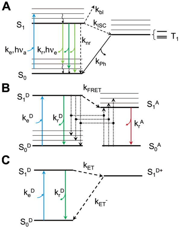
Jablonski diagrams for fluorescence, FRET and ET. (A) Upon absorption of a photon of energy hν_a close to the resonance energy E_S1 – E_S0, a molecule in a vibronic sublevel of the ground singlet state S₀ is promoted to a vibronic sublevel of the lowest excited singlet state S₁. Nonradiative, fast relaxation brings the molecule down to the lowest S₁ sublevel in picoseconds. Emission of a photon of energy hν_e < hν_a (radiative rate k_r) can take place within nanoseconds and bring back the molecule to one of the vibronic sublevels of the ground state. Alternatively, collisional quenching may bring the molecule back to its ground state without photon emission (nonradiative rate k_nr). A third type of process present in organic dye molecules is ISC to the first excited triplet state T₁ (rate k_ISC). Relaxation from this excited state back to the ground state is spin-forbidden, and thus, the lifetime of this state (1/k_Ph) is in the order of microseconds to milliseconds. Relaxation to the ground state takes place by either photon emission (phosphorescence) or nonradiative relaxation. (B) FRET involves two molecules: a donor D and an acceptor A whose absorption spectrum overlaps the emission spectrum of the donor. Excitation of the acceptor to the lowest singlet excited state is a process identical to that described for single-molecule fluorescence (A). In the presence of a nearby acceptor molecule (within a few nanometers), donor fluorescence emission is largely quenched by energy transfer to the acceptor by dipole–dipole interaction with a rate k_FRET ∼ R⁻⁶, where R is the D–A distance. The acceptor and donor exhibit fluorescent emission following the rules outlined in part A and omitted in this diagram for simplicity. (C) PET effectively oxidizes the donor molecule with a rate k_ET ∼ exp (–βR), preventing its radiative relaxation. Upon reduction, the molecule relaxes nonradiatively to its ground state. In this scheme, the electron acceptor does not fluoresce and is therefore not represented.

The existence of FRET or ET can be detected at the ensemble level by a reduction of the donor fluorescence quantum yield Φ, defined as the proportion of excitation events resulting in the emission of a fluorescence photon:

$$\Phi =\frac{k_{\text{r}}}{k_{\text{r}}+k_{\text{ISC}}+k_{\text{bl}}+k_{(\text{FR})\text{ET}}}={\Phi }_0/\left(1+\frac{k_{(\text{FR})\text{ET}}}{k_{\text{r}}}{\Phi }_0\right)$$ (1)

where k_r is the radiative relaxation rate, k_ISC the intersystem crossing (ISC) rate, k_bl is the bleaching rate, and k_(FR)ET is the FRET or ET rate, whose distance dependence is described in the next sections (Figure 1A–C). Equivalently, transfer can be detected as a decrease in the fluorescence lifetime of the donor τ:

$$\tau =\frac{1}{k_{\text{r}}+k_{\text{ISC}}+k_{\text{bl}}+k_{(\text{FR})\text{ET}}}={\tau }_0/(1+k_{(\text{FR})\text{ET}}{\tau }_0)$$ (2)

The solution of the rate equations also leads to the well-known fact that the emission F of a fluorescent molecule saturates at high excitation intensities due to the presence of a nonfluorescent triplet state:⁸⁰

$$\begin{array}{c}F=\frac{I_{\text{e}}/I_{\text{s}}}{1+I_{\text{e}}/I_{\text{s}}}{F}_{\infty }\\ I_{\text{s}}=\frac{{(\sigma \tau )}^{-1}}{1+k_{\text{ISC}}/k_{\text{ph}}}\end{array}$$ (3)

where the excitation saturation intensity I_s depends on the absorption cross-section σ, the fluorescence lifetime, and the triplet state population (k_ISC) and depopulation (k_ph) rates. I_e is the excitation intensity, and F_∞ is the maximum fluorescence rate obtained asymptotically for infinite excitation rates.

2.2. Fluorescence Polarization

The orientation of the fluorophore plays a role in both absorption and emission processes, due to their dipolar nature. The excitation rate k_e (Figure 1A) depends on the incident power, absorption cross-section σ, and relative orientation of the incident electromagnetic field E and the absorption dipole moment μ_abs:

$$k_{\text{e}}=\sigma {({\mu }_{\text{abs}}·E)}^2$$ (4)

As mentioned, the emitted intensity is proportional to the population of the excited state S₁ but also to the detection efficiency, which can be chosen to be polarization sensitive. If I_s and I_p are the collected linear polarized intensities along two perpendicular directions in a plane orthogonal to the direction of light propagation (the microscope optical axis in single-molecule measurements, see Figure 2), the (time-dependent) polarization anisotropy is defined as:^78,82–84

Figure 2.

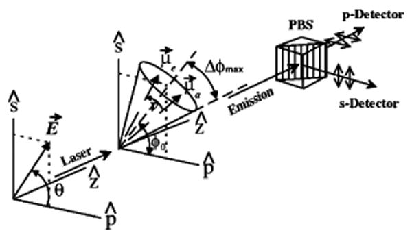
Polarization spectroscopy geometry. E⃗ is the electric field, making an angle θ with the p polarization axis. The excitation propagates along axis z, which is also the collection axis. μ⃗_a and μ⃗_e are the absorption and emission dipole moments, initially aligned. ν represents the rotational diffusion of the emission dipole during the excited lifetime. The dipole is supposed to be confined in a cone positioned at an angle φ₀ projected on the (s, p) plane and having a half-angle Δφ_max. A polarizing beam splitter splits the collected emission in two signals I_s and I_p, which are simultaneously recorded by APDs. Adapted Figure 1 with permission from ref 223 (http://link.aps.org/abstract/PRL/v80/p2093). Copyright 1998 by the American Physical Society.

$$r=\frac{I_{\text{s}}-I_{\text{p}}}{I_{\text{s}}+2I_{\text{p}}}$$ (5)

For a freely rotating molecule:

$$r(t)=\frac{1}{5}(3{cos}^2\alpha -1)e^{-t/{\tau }_{\text{r}}}$$ (6)

where α is the angle between the emission and the absorption dipole of the molecule and τ_r is the rotational diffusion time. Polarization-sensitive (time-resolved) measurements can thus yield information on the (time-dependent) orientation of the fluorophore and have been used to study DNA and protein conformations at the single-molecule level as will be reviewed later.^83–86

2.3. FRET

FRET between a donor and an acceptor molecule occurs when both are at a distance of the order of a few nanometers.⁸⁷ It is due to nonradiative Coulombic dipole–dipole interactions and is characterized by a rate k_FRET given by:^87,88

$$k_{\text{FRET}}=\frac{1}{{\tau }_0}{\left(\frac{R_0}{R}\right)}^6$$ (7)

where τ₀ is the donor fluorescence lifetime in the absence of acceptor and R₀ is the Förster radius. R₀ is proportional to the orientation factor κ², the donor–acceptor spectral overlap J (in M⁻¹ cm⁻¹ n10), and the donor quantum yield Φ_D:For donor emission and acceptor absorption dipoles

$$R_0^6=8.79\times {10}^{23}\frac{{\kappa }^2{\Phi }_{D}J}{n^4}(\text{in}{\mathring{\text{A}}}^6)$$ (8)

$${\kappa }^2={(cos{\theta }_{\text{T}}-3cos{\theta }_{\text{D}}cos{\theta }_{\text{A}})}^2$$ (9)

$$J={\int }_0^{\infty }{f}_{\text{D}}(\lambda ){\epsilon }_{\text{A}}(\lambda ){\lambda }^4\text{d}\lambda$$ (10)

rotating fast as compared to the donor fluorescence lifetime, κ² in eq 8 can be replaced by its average value 〈κ²〉, which equals 2/3 for isotropic rotation. In the general case, κ² takes a time-dependent value (eq 9), where θ_T is the angle between the donor emission dipole and the acceptor absorption dipole and θ_D (respectively, θ_A) is the angle between the donor–acceptor connection line and the donor emission dipole (respectively, acceptor absorption dipole). The spectral overlap integral J involves the normalized fluorescence emission spectrum of the donor f_D [∫f_D(λ) dλ = 1] and the molar extinction coefficient of the acceptor ε_A (in M⁻¹ cm⁻¹). Values of R₀ for common dye pairs range from 2 to 6 nm.⁸⁷ κ² is a dominant factor in distance fluctuations of the Förster radius R₀ and depends on the relative orientation of D and A dipoles. As discussed previously, FRET can be detected by measuring the change in donor lifetime (eq 2). Introducing the FRET efficiency E:

$$E=\frac{k_{\text{FRET}}}{k_{\text{r}}+k_{\text{onr}}+k_{\text{FRET}}}={\left[1+{\left(\frac{R}{R_0}\right)}^6\right]}^{-1}=1-\frac{\tau }{{\tau }_0}$$ (11)

E can also be measured ratiometrically from the donor and acceptor fluorescence intensities F_D and F_A:

$$E=\frac{F_{\text{A}}}{F_{\text{A}}+\gamma F_{\text{D}}}$$ (12)

where γ incorporates the donor and acceptor quantum yields (Φ) and the detection efficiencies of both channels (η):

$$\gamma =\frac{{\eta }_{\text{A}}{\Phi }_{\text{A}}}{{\eta }_{\text{D}}{\Phi }_{\text{D}}}$$ (13)

FRET measurements, performed by donor lifetime measurement or ratiometric measurement of the donor and acceptor emissions, are therefore sensitive to the donor–acceptor distance and/or respective orientations. The use of FRET as a “spectroscopic ruler” was first proposed and demonstrated by Stryer and Haugland⁸⁹ at the ensemble level and has been extensively used ever since to measure intermolecular interactions and to study molecular conformations and environments. These applications were later extended to the single-molecule level,^90,91 and FRET is now a workhorse of single-molecule spectroscopy.

2.4. Single-Molecule ET

ET between a donor and an acceptor molecule occurs at a rate k_ET that depends on two main factors: the coupling between the reactant and product electronic wave functions V_R² and the Franck–Condon weighted density of states FC.^92,93 The latter is usually constant for macromolecules; therefore, one is left with the electronic coupling term, which depends exponentially on the distance between donor and acceptor:

$$V_{\text{R}}^2=V_0^{2}exp(-\beta R)$$ (14)

where β has been measured for different systems to vary from 1.0 to 1.4 Å⁻¹ in proteins. The ET rate k_ET can be accessed by measuring the donor fluorescence emission or the donor fluorescence lifetime, assuming that no other process influences these two observables. Fluorescence quenching by ET can be used to monitor minute conformational changes in biopolymers as it requires close contact between the donor and the acceptor molecules. This approach has been used at the single-molecule level to study dye-labeled polypeptides containing a tryptophan residue⁹⁴ and a flavin reductase enzyme in which the fluorescence of an isoalloxazine is modulated by photoinduced electron transfer (PET) to a tyrosine.⁹⁵

This brief overview of some of the photophysical characteristics of fluorophores used in single-molecule spectroscopy has illustrated theoretically how sensitive the absorption and emission can be to the local environment of the fluorophore. Therefore, any modification or fluctuation of fluorescence intensity or lifetime (the two main observables) observed in an experiment should be carefully analyzed to exclude genuine photophysical effects that have nothing to do with potential intra- or intermolecular changes of the macromolecule to which the fluorophore is attached. Simple controls such as studying the excitation power dependence of the observed effect and analysis of the photophysics of the dye alone or of singly labeled macromolecules in the case of FRET studies are necessary to ascertain the physical origin of the observable variation (see, for instance, ref 96).

3. Single-Molecule Data Acquisition and Analysis Methods

The basic experimental principle and design of single-molecule spectroscopy reviewed during the past few years^3–7 have remained mostly unchanged, even if some technological improvements have surfaced, from multiple laser excitation schemes to better detector sensitivity and faster acquisition electronics. Indeed, the most important recent developments have involved developing new fluorophores and new labeling schemes (reviewed in ref 97) providing more versatile tools for the study of specific molecules, investigation of more complex biological systems, and elaboration of sophisticated data analysis tools. We will first review here the novel methods that have been developed since and illustrate their utilization with a few examples, leaving the bulk of actual biological results to the corresponding sections of this article.

3.1. Single-Molecule Fluorescence Experimental Setups

3.1.1. General Considerations

Numerous books and reviews are available for detailed descriptions of experimental designs for single-molecule fluorescence spectroscopy and microscopy.^{1–5,7,80,84,98–102} We will limit ourselves to describe schematically the two typical geometries that are commonly used, confocal microscopy and wide-field microscopy (Figure 3). The use of a high numerical aperture objective is mandated by the need to tightly focus the excitation light in order to reduce the excited volume to a minimum and to collect as much as possible of the few photons emitted by a single molecule. Reduction of the excitation volume helps lowering background and, therefore, enhances the signal-to-background level. Despite the use of high-efficiency filters and dichroic mirrors, as well as high-sensitivity detectors [avalanche photodiodes (APDs) in confocal microscopy or cooled intensified or nonintensified cameras in wide-field microscopy], the final collection efficiency of such setups remains typically below 10%. Confocal geometries and their associated fast detectors allow high-temporal resolution recording [down to a few dozens of ps in time-correlated single-photon counting (TCSPC) techniques] and are ideally adapted to the study of diffusing molecules (Figure 3A,B). The number of detectors can vary greatly depending on the number of parameters recorded and can reach four APDs for dual-color, two-polarization recording, enabling intensity, lifetime, polarization anisotropy, and spectral identity to be collected simultaneously. ^103–105 Wide-field geometries, and especially total internal reflection (TIR) (Figure 3C–E), are principally limited to surface studies of either surface-bound or membrane-embedded molecules. The corresponding detectors are typically capable of transferring from tens to hundreds of frames or regions of interest per second with minor readout noise but are not single-photon counting devices. Dual-color and/or dual-polarization spectral studies, first suggested by Kinosita's group,¹⁰⁶ can be performed by a judicious use of the detector area as illustrated on the right-hand side (RHS) of Figure 3E.^107,108 Two-dimensional photon-counting devices are currently plagued by low count rates and detection efficiency but may become attractive single-molecule detectors in the future.¹⁰⁹

Figure 3.

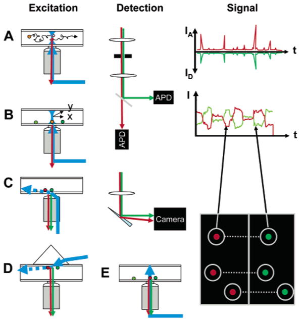
Experimental geometries in single-molecule fluorescence spectroscopy. Two main types of geometries can be used for single-molecule fluorescence spectroscopy: confocal and wide field. In the confocal geometry (A, B), a collimated laser beam is sent into the back focal plane of a high numerical aperture objective lens, which focuses the excitation light into a diffraction limited volume (or point spread function, PSF) in the sample. PSF engineering can be used at this stage to shape the excitation volume in order to gain resolution in any dimension. Fluorescence emitted by molecules present in this volume is collected by the same objective and transmitted through dichroic mirrors, lenses, and color filters to one or several point detectors (APD). An important aspect of this geometry is the presence of a pinhole in the detection path, whose size is chosen such as to let only light originating from the region of the excitation PSF reach the detectors. Freely diffusing molecules (A) will yield signals comprised of bursts of various size and duration (but typically less than a few milliseconds), as indicated schematically on the RHS. Immobile molecules (B) will need to be first localized using a scanning device (indicated as two perpendicular arrows x and y), before recording can commence. Typical time traces are comprised of one or more fluctuating intensity levels until the molecule eventually bleaches after a few seconds, as indicated schematically on the RHS. The wide-field geometry (C–E) can be used in two different modes: (C, D) TIR or (E) epifluorescence. In TIR, a laser beam is shaped in such a way that a collimated beam reaches the glass–buffer interface at a critical angle θ = sin⁻¹(n_buffer/n_glass), where n designates the index of refraction. This creates an evanescent wave (decay length of a few hundreds of nanometers) in the sample (dashed arrow), which only excites the fluorescence of the molecules in the vicinity of the surface, resulting in a very low background. TIR can be obtained either with illumination through the objective (C) or by coupling the laser through a prism (D); both methods have their advantages and inconveniences (for details, see ref 224). In epifluorescence (E), a laser beam focused at the back focal plane of the objective or a standard arc lamp source is used to illuminate the whole sample depth, possibly generating additional background signals. A wide-field detector (camera) is used in all three cases, allowing the recording of several single-molecule signals in parallel, although with a potentially smaller time resolution than that achieved with point detectors. The image on the RHS represents the case of a dual-color experiment, where both spectral channels are imaged simultaneously on the same camera (signals from the same molecule are connected by dotted line). Individual intensity trajectories can be extracted from movies, resulting in similar information as that obtained with the confocal geometry.

As discussed later and illustrated in the RHS of Figure 3, the signals obtained from all of these different types of experiments (such as donor and acceptor intensities in the case of FRET experiments, fluorescence lifetime, or fluorescence polarization anisotropy for time-resolved studies) are eventually reduced to time traces of one or more observables, histograms of these observables, or auto- or cross-correlation functions (CCFs).

3.1.2. Multiple Laser Excitations

Traditional single-laser excitation studies performed in solution or with surface-immobilized molecules have in common that the FRET efficiency (E) histograms collected from such experiments are contaminated by a zero-E, or D-only, peak.^70,91,110 The D-only peak may arise from fluorescence bursts with D-only emission (e.g., proteins with D-only due to incomplete labeling), complex photophysics (e.g., acceptor bleaching), formation of long-lived nonfluorescent triplet states resulting in dark (or off) states, and/or contributions from solvent. The presence of the D-only peak interferes with distributions of subpopulations in the low-E region (E < 0.4) and complicates the extraction of mean E values, distribution width, or relative weights of subpopulations analysis from the E histogram.

In order solve this problem, Kapanidis et al. have recently introduced an alternating-laser excitation (ALEX) scheme, during which one switches between D excitation (λ_D) and direct A excitation (λ_A) at a microsecond time scale, faster than the diffusion time of a protein through the detection volume (for small globular proteins of < 10 kDa ∼ 1 ms).¹¹¹ Microsecond ALEX (μs-ALEX) spectroscopy allows the recovery of distinct emission signatures for all diffusing species (Figure 4A). For each single-molecule burst, the number of photons emitted from D upon $(F_{{\text{D}}_{\text{exc}}}^{{\text{D}}_{\text{em}}})$, the number of photons emitted from A upon D excitation $(F_{{\text{D}}_{\text{exc}}}^{{\text{A}}_{\text{em}}})$, and the number of photons emitted after direct excitation of A $(F_{{\text{A}}_{\text{exc}}}^{{\text{A}}_{\text{em}}})$ are counted. Sorting of subpopulations is achieved with the help of a 2D histogram (Figure 4B) by calculating two ratios: The traditional FRET efficiency ratio E, defined as:

Figure 4.

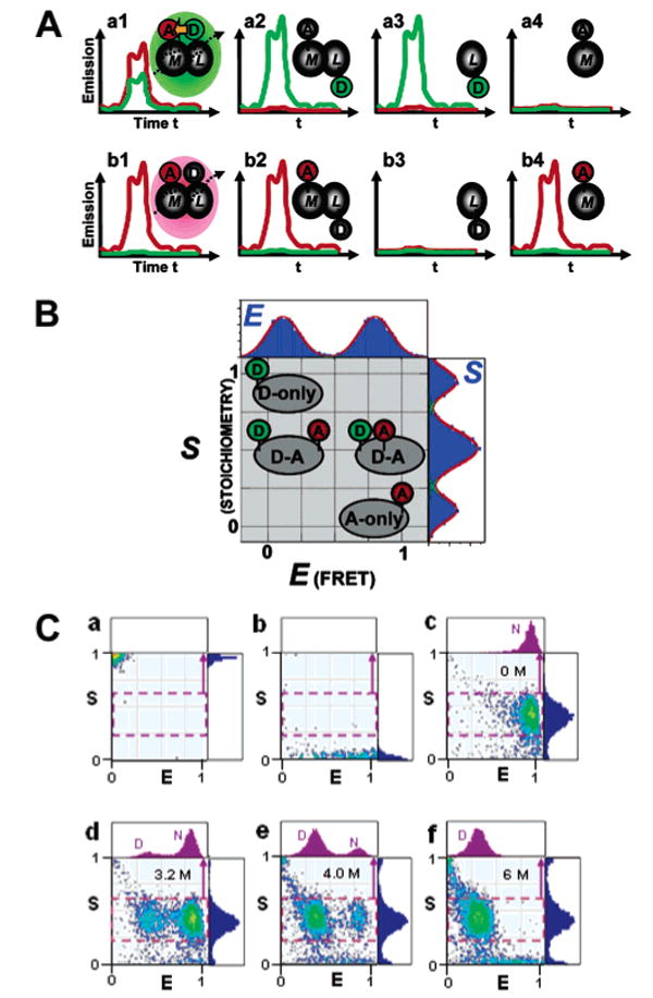
Fluorescence-aided molecular sorting using μs-ALEX. ALEX allows detection of D excitation- and A excitation-based fluorescence emission for single diffusing molecules, enabling fluorescence-aided molecular sorting. The advantages of ALEX over traditional single-laser excitation is exemplified in part A, using the interaction between a D-labeled ligand (L) and an A-labeled macromolecule as an example (D and A depicted as green and red ovals, respectively). The top panel shows emission caused by D-excitation using single-laser excitation. Short distances within the M–L complex cause emission predominantly in the acceptor channel (red curves), whereas large distances mainly result in D emission. Note that there is no discrimination between a low-FRET complex and the fluorescence emission signature resulting from unbound L, and free M is not detectable. ALEX allows direct excitation of the A, allowing one to distinguish between low-FRET complexes and unbound acceptor. (B) Two-dimensional E–S histogram for single-molecule sorting. The conventional FRET efficiency E sorts species according to D–A distance and thus reports on structure. The novel stoichiometric ratio S reports on D/A stoichiometry. The additional dimension allows D-only and A-only species to be distinguished from low- and high-FRET subpopulations, respectively. (C) ALEX-based probing of the equilibrium unfolding of CI2, specifically labeled with Alexa647 at the N terminus and Alexa488 at position 40. Representative 2D E–S histograms of D-only-labeled CI2 (a), A-only-labeled CI2 (b) and D/A-labeled CI2 at various concentrations of GdmCl (c–f). One-dimensional histograms of the stoichometric ratio S are shown in blue color to the right of each histogram. One-dimensional histograms of the FRET efficiency E for each sample are displayed on top of each 2D histogram in purple. See the text for details. Parts A and B are adapted with permission from ref 111. Copyright 2004 National Academy of Sciences U.S.A. Part C is reprinted with permission from ref 173. Copyright 2005 Cold Spring Harbor Laboratory Press.

$$E=F_{{\text{D}}_{\text{exc}}}^{{\text{A}}_{\text{em}}}/(F_{{\text{D}}_{\text{exc}}}^{{\text{A}}_{\text{em}}}+\gamma F_{{\text{D}}_{\text{exc}}}^{{\text{D}}_{\text{em}}})$$ (15)

and the novel distance-independent stoichometric ratio S, defined as:

$$S=F_{{\text{D}}_{\text{exc}}}/(F_{{\text{D}}_{\text{exc}}}+F_{{\text{A}}_{\text{exc}}})$$ (16)

where the absence of upper indices indicates that all signals are summed. While E reports on D–A distances, and thus indirectly on structure within labeled molecules, S reports on D–A stoichiometry. If the excitation power is tuned such that the average D excitation-based emissions (F_Dexc) equal the average A excitation-based emissions (F_Aexc), E will adopt a value of E ∼ 0 and S ∼ 1 for D-only samples whereas for A-only samples, E ∼ 1 and S ∼ 0. In a D/A-labeled sample, E can assume any value between 0 and 1 and the S ratio will be ∼0.5.¹¹¹ The ability to colocalize D and A fluorophores on a single molecule allows one to distinguish zero-FRET from D-only populations and thus extend FRET-based distance measurements to 0% FRET efficiencies, eliminate contributions from the buffer, evaluate binding stoichiometries and complex composition, and quantitate the effect of local environment without FRET constraints. ALEX can be achieved over a broad range of time scales from the nanosecond time scale (to extract distance distributions within subpopulations and dynamic information on the 1–100 ns time scale, see below) to the millisecond time scale in studies with surface-immobilized proteins to process raw E trajectories by removing time points with inactive acceptor (reviewed in ref 112).

A related but different approach developed recently by Klenerman and collaborators¹¹³ uses two (nonalternating) lasers with partially overlapping excitation volumes, effectively reducing the region where the two corresponding fluorophores are simultaneously excited. This volume reduction decreases the background proportionally more than the signal level, which results in an enhanced signal-to-noise ratio after selection of only single-molecule bursts exhibiting both signals. From the signals coming from the two fluorophores excited by the two lasers, a stoichiometric ratio related to S defined in eq 16 can be computed, whose autocorrelation function (AF) is then devoid of any diffusion component (as both dyes exhibit the same diffusion pattern, being attached to the same molecule). Analysis of the ratio AF thus gives access to submicrosecond fluctuation dynamics of one (or both) fluorophore emission. Li et al. have used this approach with fluorophores not undergoing FRET to study DNA hairpin dynamics as a benchmark and have discovered submicrosecond dynamics of a RNA region of a dimerized human telomerase.¹¹³ Provided that intramolecular dynamics results in quenching of the fluorophore (resulting in intensity fluctuations), this technique should be applicable to other biological macromolecules, such as proteins.

Nanosecond-ALEX (ns-ALEX) is the latest addition to the toolbox of ALEX-based spectroscopies.¹⁰⁵ In ns-ALEX, interlaced, picosecond pulses from two synchronized mode-locked lasers are used to obtain 14.7 ns alternation periods in conjunction with fluorescence lifetime measurements (Figure 6A). A related approach was also independently presented by Müller et al.¹¹⁴ In the setup described by Laurence et al., excitation is linear-polarized and four detection channels are employed that allow the separation of emission according to polarization and D and A spectra. As described in detail for μs-ALEX,¹¹¹ for each diffusing single molecule, the number of photons emitted from D and from A (emitted after direct A excitation or emitted after D excitation via FRET) is counted, and ratios of FRET efficiencies (E) and D/A stoichiometries (S) are calculated (Figure 6B). In addition to its capability of fluorescence-aided molecular sorting into subpopulations (D-only, A-only, and D/A-labeled), ns-ALEX also provides access to time-resolved FRET and time-resolved fluorescence anisotropy, which are unavailable to μs-ALEX. Two time measurements are made for each photon: (i) the time since the experiment began (macrotime t) and (ii) the time delay between a donor excitation pulse and a photon (microtime τ) (Figure 6A). Single molecules on transit through the confocal detection volume are identified by t, while τ is used to determine fluorescence lifetimes and assign correct laser excitation to a photon. The option for time-resolved measurements has several advantages. First, as mentioned above, accurate FRET efficiencies can be calculated directly from measurements of the D lifetime. Because such measurements involve a single chromophore and a single detector, no correction factors are needed. Second, multiexponential fluorescence lifetime decays can be analyzed to identify distance distributions and conformational fluctuations on time scales down to the D lifetime within subpopulations (e.g., denatured states of proteins) (Figure 4C). Third, rotational freedom of fluorophores can be scrutinized and the orientation factor κ² (eq 9) can be estimated more accurately.

Figure 6.

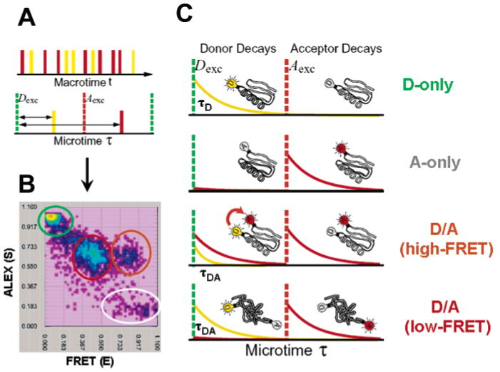
Principle of ns-ALEX. (A) Interlacing pulses from two lasers, D_exc (green, excites D) and A_exc (red, excited A), with a fixed delay between the detected photons; the D_exc laser pulse is measured with ∼500 ps resolution, providing information about fluorescence lifetime and the ability to classify photons according to D_exc or A_exc (i.e., whether time delay τ is before or after the A_exc pulse). (B) Two-dimensional E–S photon burst histogram resulting from single molecules of D/A-labeled CI2 diffusing through the laser focal spot in the presence of 4 M GdmCl. Values for the FRET efficiency E and stoichiometry ratio S are calculated and placed in a 2D E–S histogram. Four species are detected as follows: D only (green circle), A only (grey circle), folded CI2 (high-FRET) (orange circle), and denatured CI2 (low-FRET) (red circle). The corresponding time-resolved fluorescence decay curves are extracted from the relevant portions of the photon stream and are depicted in part C. D-only molecules emit only after D excitation (yellow curve, leakage into the A channel removed for clarity), while A-only molecules only emit after A excitation (red trace). Unfolded proteins labeled with D and A emit D and A fluorescence after a D_exc pulse (ratio of intensities and lifetimes depend on FRET efficiency) and emit A fluorescence after A_exc. Folded proteins labeled with D and A emit similarly, except with a higher relative intensity of A as compared to D after the D excitation pulse and with a shorter D lifetime, indicating a higher FRET efficiency due to shorter average distance.

3.1.3. Accurate FRET Efficiencies Measurements

FRET efficiencies at the single-molecule level can be measured by sensitized A emission (the ratiometric E approach)^91,115 or by changes in D lifetime¹⁰³ as discussed previously. While the D lifetime-based method has been until recently technically demanding and requires relatively sophisticated and expensive instrumentation, it allows E determination directly from the D lifetime decay rates using D-only and D/A-labeled samples. However, recent progresses in timing electronics integration and pulsed laser diode technology have made this approach more accessible.^116,117 The ratiometric E method, on the other hand, is easy to implement, but accurate E determination requires a detailed knowledge of the correction factor γ, which depends on D and A quantum yields, detection efficiencies for D and A emission, optical alignment and filters used, solvent conditions (temperature, pH), and possibly other unknown factors. Accurate E measurements at the single-molecule level thus require three main corrections: (i) separation of D leakage from FRET-induced A emission, (ii) separation of A direct excitation from FRET-induced A emission, and (iii) corrections for differences in the quantum yield and detection efficiency of the fluorophores (factor γ, eq 13).

Using the ratiometric E method, Ha et al. determined γ by photobleaching of surface-immobilized molecules.¹¹⁸ Unfortunately, γ obtained in this way is only an approximation when used in solution experiments, due to possible surface-induced changes in fluorophore photophysics and possible chromatic differences in the detection volume on surfaces and in solutions.

As pointed out by Lee et al.,¹¹⁹ ALEX offers a convenient way to obtain these correction factors directly and simultaneously with measurements of FRET efficiencies. For example, the correction factor for D leakage can be obtained from the D-only subpopulation by normalizing D excitation-based A emission with D excitation-based D emission (factor l, Figure 5A). A correction factor for the A-only subpopulation can be obtained similarly (factor d, Figure 5A). Corrected E and S values are then obtained by subtracting the contributions from l and d from the experimental data in the photon stream. Finally, the reprocessed E values are plotted over 1/S, to obtain correction factor γ from the slope of the plot. Because ALEX allows these correction factors to be obtained directly and simultaneously with FRET efficiencies, ALEX-based distances are independent of instrument-specific factors, such as excitation intensity or detector alignment.

Figure 5.

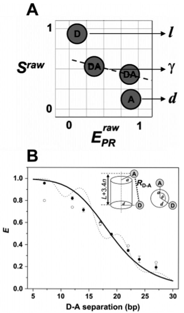
Application of μs-ALEX for accurate FRET measurements in biomolecules at the single-molecule level. (A) Species required for recovering all correction factors needed for accurate ratiometric E measurements. D-only species provide the D leakage factor l, A-only species provide the A direct excitation factor d, and two D–A species with a large difference in E provide the correction factor γ. (B) Comparison of E values measured for DNA fragments with values predicted from cylindrical models of DNA. ALEX-based E values (filled black dots) and E values from ensemble measurements (open circles) are shown. The solid black curve represents the theoretical dependence of the E value on D–A separation with the D probe proximal to the DNA helical axis, while the dotted line represents theoretical E values with the D probe distal from the DNA helical axis. Note that in all cases, a single-molecule-based E value fit better to theoretical values than ensemble-based values. Adapted with permission from ref 119. Copyright 2005 Biophysical Society.

Using double-stranded (ds) DNA fragments as model systems, Lee et al. further showed that ALEX-based intramolecular DNA distances agree well with predictions made from a cylindrical model of helical DNA, even better than distance estimates made from ensemble FRET data (Figure 4B). In addition, single-basepair (bp) resolution in ALEX was confirmed by using a set of dsDNA fragments that featured 15, 16, or 17 bp separations between the D and the A, and measurements within RNA–polymerase–DNA transcription complexes yielded distances in agreement with ensemble FRET measurements and with models based on systematic FRET studies using multiple transfer efficiencies as distance constraints and X-ray crystallography. Thus, ALEX can complement structural analysis of biomolecules that are intractable or difficult to study by conventional structural biology due to heterogeneity, limited stability or solubility, large size, flexible domains, or transient nature.

3.1.4. Three-Color FRET

Two-color single-molecule FRET is an important experimental tool to probe biological processes directly without temporal and population averaging of ensemble experiments. For more complex systems, however, a single distance reporter may not be sufficient for a complete understanding of the underlying molecular dynamics (MD) and conformational changes. A solution to this problem is the addition of a third fluorophore, which allows the measurement of three distances. Three-color FRET has been demonstrated recently by several groups on the ensemble level^120–122 and, more recently, at the single-molecule level. Ha and co-workers employed three-color FRET to study conformational dynamics in the DNA four-way (Holliday) junction,¹²³ while Clamme and Deniz¹²⁴ used a simpler, rigid DNA duplex scaffold as a model system.

The ALEX concept was recently extended to include a third alternating laser (488, 543, and 638 nm light) (three-color ALEX) for the accurate and simultaneous measurements of three interdye distances in freely diffusing biomolecules labeled with three different fluorophores [Alexa Fluor 488 (donor), Alexa Fluor 546 (acceptor 1), and Alexa Fluor 647 (acceptor 2)] (Lee et al., unpublished results). Three-color ALEX has been demonstrated using a triply labeled dsDNA fragment. To demonstrate the robustness of three-color ALEX, the dsDNA molecule was hybridized from three chemically synthesized, singly labeled single-strand (ss) DNA fragments, yielding up to seven possible species (three singly labeled species, three doubly labeled species, and the triply labeled fragment). Sorting of the labeled species and identification of the triply labeled subpopulation were achieved in 2D S_i−S_j histograms, where S_i is a new stoichiometry ratio aimed at separating different species. The selected subpopulation of triply labeled dsDNA was then analyzed for the three interdye FRET efficiencies using the relevant data in the photon stream. The FRET efficiencies calculated from the corrected FRET efficiencies were in good agreement with the theoretical values expected assuming a cylindrical DNA model. Three-color ALEX can thus be useful for the simultaneous probing of three distances in a polypeptide chain (e.g., to dissect the order of domain unfolding in a protein or to address complex kinetics by timing sequential and concerted changes in stoichiometry and/or distance during a multistep process). Extension to a four-color implementation (allowing, in principle, up to six distances within a single molecule) is possible by taking advantage of a spectral window between tetramethylrhodamine (TMR) and Alexa Fluor 647 that can be invoked to introduce a fourth fluorophore (e.g., Alexa Fluor 594). In fact, a recent single-molecule demonstration of five-color FRET has been reported in a model photonic wire system comprised of short DNA strand-labeled with five fluorophores.¹²⁵

3.2. Data Analysis Methods

3.2.1. General Considerations

Conformational dynamics studies are concerned with three fundamental questions: (i) identification of the different conformational states explored by the molecule, (ii) quantification of the transition rates between those states, and (iii) identification of transition pathways, correlations or memory effects, or variable kinetic constants in the time trajectory. Fluorescence spectroscopic methods explore these questions via the measurement of temporal evolution of fluorescence observables (spectrum, lifetime, polarization anisotropy, FRET efficiency, etc). These observables are indirect signatures of the underlying conformational evolution of the molecule, as discussed in a previous section (fluorescence spectroscopy). In practice, the collected signal is contaminated by contributions from various unrelated photophysical phenomena (background, triplet state blinking, bleaching, etc). They need to be identified, and their contribution needs to be quantified, as they can introduce new states and rates and, therefore, affect time trajectories. Initial attempts to study conformal dynamics of individual proteins have taken the natural (although nontrivial) route of surface immobilization, the rationale being that an immobile molecule can be observed for a long period of time (up to tens of seconds).^118,126,127 However, subsequent studies have rapidly documented the drawbacks of this approach, namely, the numerous artifacts resulting from modification of the molecule with some chemical moiety or additional peptide sequence for attachment to the surface or, more problematically, because of interactions between the molecule and the surface. To avoid these problems, particularly acute in protein experiments, a number of studies have tried to extract information on protein conformational dynamics from diffusing molecules. The discrete stream of photons detected during these experiments can be analyzed simply in terms of burst intensities or any other observable such as lifetime, polarization anisotropy, FRET efficiency, etc., measured during each burst.

As experimental techniques have approached the limits of currently accessible sensitivity, number of measurable parameters, and time resolution, a large part of recent developments in single-molecule fluorescence spectroscopy of protein conformational dynamics has thus dealt with data analysis methods that could extract information from the collected photon streams most efficiently.

3.2.2. Photon Stream and Time Traces

Historically, both wide-field and confocal experiments have represented the collected signal as time-binned traces. In the case of wide-field detection, this is imposed by the way cameras collect photons, namely, by integration of the emitted signal during a finite period of time before transfer. In confocal experiments, the use of photon-counting detectors does not impose such a binning, but the original and still most convenient way to represent the raw data is by binning the detected photon in such a way as to have a sufficient signal-to-noise ratio (a few tens of photons or more per bin during emission). For typical detected signals of a few tens of kilohertz, bin sizes of less than a few hundreds of microseconds result in a noisy signal.

Conformational changes can be detected if they result in fluctuations of the emitted fluorescence intensity or lifetime (by quenching, FRET, ET, or a change in the polarization anisotropy). The most appropriate approach to detect these fluctuations will depend on the respective time scales of the fluctuations τ_f, the time resolution of the measurement δτ_r, and the geometry of the experiment, which will in general set a typical time duration T for each observation. The time resolution of the measurement δτ_r can be defined in several ways. Here, we will use the lower bound δτ_r ∼ 1/s, where s is the signal count rate, which results in a signal-to-noise ratio of 1.

For diffusion experiments, in which each molecule transits briefly through the excitation volume generating a burst of fluorescence (transit time T ∼ 1 ms or less), conformational changes occurring at time scales larger than T (δτ_r < T ≪ τ_f) will be detected by the presence of different burst subpopulations characterized by distinct values of the observable (lifetime, FRET efficiency, etc). This is due to a low probability of occurrence of a transition during the typical transit time. This regime is reviewed in detail in the section on equilibrium studies.

3.2.3. FCS

Conformational changes at a very fast time scale (τ_f ≪ δτ_r < T) will usually not be resolvable from a simple histogram of the binned observable and will require time correlation techniques across many bursts (FCS^128–130 or related approaches, such as photon counting histogram (PCH),¹³¹ fluorescence multiple intensity distribution analysis (FIMDA),¹³² or photon arrival-time interval distribution (PAID)¹³³), to acquire enough statistical information on the transitions from multiple single-molecule events.

In FCS, the AF of the fluorescence intensity I(t):

$$G\left(\tau \right)=\frac{\langle I\left(t\right)I\left(t+\tau \right)\rangle }{\langle I\left(t\right)\rangle \langle I\left(t+\tau \right)\rangle }$$ (17)

is computed for all accessible time lags τ and 〈 I(t) 〉 = 〈 I(t + τ)〉 for a stationary process. Characteristic time scales of the fluorescence fluctuations appear in the fitted form of the AF. In the case of free diffusion of a two-state fluorophore (Figure 1A with no triplet state) diffusing in a 3D Gaussian excitation volume of widths w_xy and w_z:

$$G\left(\tau \right)=1+\frac{1}{N}{\left(1+\frac{\tau }{{\tau }_{\text{D}}}\right)}^{-1}{\left(1+\frac{\tau }{{\omega }^2{\tau }_{\text{D}}}\right)}^{-1/2}$$ (18)

where N is the number of particles in the observation volume, τ_D is the diffusion time of the particle (τ_D = w_xy²/4D), and ω = w_z/w_xy is the height-to-diameter ratio of the 3D Gaussian confocal volume. In the presence of a triplet state, or any other type of configuration or process resulting in a change of fluorescence emission, the shape of the AF is changed into:

$$G\left(\tau \right)=1+\frac{1}{N}{\left(1+\frac{\tau }{{\tau }_{\text{D}}}\right)}^{-1}{\left(1+\frac{\tau }{{\omega }^2{\tau }_{\text{D}}}\right)}^{-1/2}·\left[1+\frac{A}{1-A}exp\left(-\tau /{\tau }_{\text{R}}\right)\right]$$ (19)

where τ_R is the relaxation time of the dynamic process and A is its amplitude. When several observables are measured simultaneously, CCFs of these observables can be measured, giving access to the time scales of correlated variation of these quantities (for instance, donor and acceptor intensity in FRET).

An approach giving access to the subnanosecond regime relevant for fast side chain fluctuations has recently been demonstrated with DNA hairpins, using TCSPC techniques borrowed from photon antibunching studies.^134,135 A similar approach was also used to address submicrosecond time scale dynamics in small polypeptides, as will be discussed later.⁹⁴

3.2.4. Time Trace Analysis

At an intermediate time scale (τ_f ∼ δτ_r < T), bursts will still be comprised of a mixture of fluorescence emission in different states, resulting in intermediate observable values. In simple model systems, it may be possible to extract information on the number of states and the time scales of interstate transitions by model-fitting the histogrammed observable values.^136,137 However, in the general case where the time scale of the fluctuations is very close to the time resolution, it is extremely difficult to extract reliable information from a simple analysis of the observable time trace.

For immobilized molecules, or very slowly diffusing molecules (e.g., trapped in vesicles¹³⁸), conformational changes will be measurable without time-correlation techniques down to ∼δτ_r, but more importantly, fluctuations with time scales above the millisecond (the usual diffusion time in a confocal spot) may have a chance to be observed, either directly on the binned trace^104,138 or using time-correlation techniques on single-molecule signals provided that the molecule does not bleach prematurely.^31,126,139

A critical issue common to both diffusing and immobilized molecule analyses is the choice of binning parameter (or time resolution δτ_r), to detect the existence and measure the value of observable states down to the lowest possible time scale. This problem is illustrated in Figure 7, which shows that simple histogramming techniques can give a hint of the existence of multiple states but are usually not sufficient to resolve them, let alone extract transition rates due to shot noise. Diverse methods have recently been proposed to deal with this problem more or less efficiently.

Figure 7.

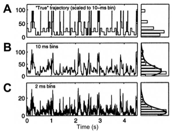
Time trace of a multistate single-molecule observable (photon counts). (A) Exact sequence of transition between states displayed with a time resolution allowing each transition to be readily observable. The histogram of intensity levels represented on the RHS exhibits five distinct states. (B) Real signal simulated by adding shot noise to the previous trace. Although indication of several levels is apparent from the various peak heights, the histogram on the RHS renders their indentification impossible. (C) Increasing the time resolution of the time trace 5-fold does not improve the situation, as shot noise becomes proportionally more important. Adapted with permission from ref 145. Copyright 2005 American Chemical Society.

Haran and collaborators^138,140 borrowed nonlinear filtering methods from the single-ion channel-recording field¹⁴¹ to extract fast transitions and small amplitude fluctuations in noisy FRET signals from vesicle-trapped adenylate kinase (AK) enzymes. The rather high level of noise in their experiment was the result of the low excitation power (300–600 nW at 488 nm) used in order to postpone fluorophore bleaching and thus obtain long time traces. This approach validated by numerical simulations was highly successful and allowed them to uncover specific features of the folding energy landscape of this protein, as discussed in a later section.

This method is hardly applicable to diffusing molecules due to the very short residence time of any molecule in the excitation volume. Ordinarily, diffusion experiments are analyzed in terms of distributions of the average observable values during individual bursts. Distributions that appear larger than expected from shot noise only¹⁴² can indicate a heterogeneous population of molecules having different static values of this observable (e.g., FRET efficiency, E) or a population of molecules fluctuating between different values.

One way of approaching this question was introduced by the Seidel group, who formed histograms of E calculated over 500 μs bins within bursts of diffusing syntaxin 1, a SNARE family protein involved in membrane fusion, known to exist in two distinct conformations, closed and open.¹⁰⁴ The result was a clearly bimodal distribution indicating fluctuations between two distinct states within bursts. Occasionally, some rare bursts can last several milliseconds, during which fluctuations can possibly be observed directly. The large shot noise value in these long bursts required the use of a maximum likelihood approach to reconstruct the most probable donor–acceptor distance trajectory R(t) explaining the observed sequence of detected photons, independent of any experimental binning, assuming a random walk diffusion of the donor–acceptor distance.^104,143 A more general maximum likelihood approach was recently formulated and numerically tested by Watkins and Yang for immobile molecules (constant excitation intensity) using Fisher information theory, eliminating the need to resort to binning or an underlying model for the dynamics altogether.¹⁴⁴ This approach was extended to the problem of detection of intensity change steps in immobile molecules, extracting the maximum information from each individual photon.¹⁴⁵ Talaga and collaborators have followed a different statistical approach to attack the problem of kinetic rate extraction from immobile single-molecule data using hidden Markov models.¹⁴⁶ Both methods indicate that surprisingly fast phenomena (as compared to the signal detection rate) could in principle be detected and measured. Although lacking any published experimental realization as of this writing, these new approaches could help discover phenomena inaccessible to the classical binning and histograming approaches.

4. Single-Molecule Fluorescence Studies of Protein Folding and Conformations at Equilibrium

The ability of SMD to separate signals from different conformations of a molecule (e.g., folded and unfolded) and to quantify their respective proportion under conditions of their coexistence can be exploited to study several problems that would otherwise hardly be addressable at the ensemble level. In protein folding, single-molecule fluorescence studies give access to the structure and conformational changes in the denatured subensemble, polypeptide chain collapse under a variety of solvent conditions, and thermodynamic parameters of the unfolding process. In enzyme activity, careful single-molecule fluorescence experiments can recover all kinetic constants of the reaction but also explore their static and dynamic heterogeneity, unravel the existence of diverse conformers, and probe the conformational energy landscape. We will review in detail a few recent case studies, which illustrate the power of single-molecule approaches, and briefly survey the growing amount of work using these methods.

4.1. Equilibrium Unfolding Studies on Simple Model Two-State Folders

4.1.1. Chymotrypsin Inhibitor 2 (CI2)

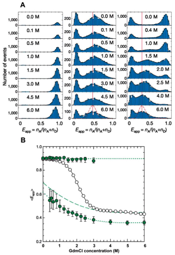
The folding mechanism of CI2 has been extensively studied experimentally at the ensemble level and by theory and simulation.^{36,42,147–156} CI2 unfolds according to a simple two-state process, with transitions between the folded and the denatured macrostates occurring on a millisecond to second time scale. Because of the simplicity of the folding mechanism of CI2 and a plethora of available thermodynamic and kinetic data from more than 100 sequence variants, CI2 is an excellent model system for benchmarking new methodology and was one of the first proteins studied at the single-molecule level.

In the study of Deniz et al.,¹¹⁰ site-specific labeling of CI2 was accomplished via chemical synthesis of the polypeptide chain using conformationally assisted native ligation.^157,158 Synthesis by parts was facilitated by the tendency of two nonoverlapping peptide chains to assemble into a nativelike complex with micromolar affinity.^154,159 Equilibrium unfolding of TMR/Cy5-labeled CI2 was studied with freely diffusing molecules in solution and an inverted confocal microscope, coupled to a high-sensitivity detection setup. The solution-based data acquisition format, which is achieved by inserting a pinhole in the image plane of the microscope to reject out-of-focus light, minimizes surface-induced artifacts on the energy landscape^127,139 and allows fast acquisition of statistically significant amounts of data.⁹¹ However, the relatively short residence time of the diffusing molecules in the excitation volume restricts the time window to obtain dynamic information in small proteins of the size of CI2 to <1 ms. After excitation of the D, emissions from the D and A were collected separately but simultaneously, and FRET efficiencies E = 1/(1 + γ F_D/F_A) (where γ is defined by eq 13) were calculated. Below 3 M GdmCl, CI2 is fully folded and the distribution of the FRET efficiency E is unimodal (mean E ∼ 0.95) (Figure 8). At intermediate denaturant concentrations, where both native and unfolded conformers coexist, an additional subpopulation (mean E ∼ 0.6) is visible, consistent with the apparent two-state folding behavior of CI2 at the ensemble level. With increasing denaturant concentrations, the relative peak ratio shifts in favor of the low-FRET peak. Above 5 M GdmCl, only the low FRET-peak is visible. The assignment of the high-FRET and low-FRET peaks to native and denatured CI2 was confirmed by using a destabilized variant of CI2. The same two peaks were observed, but at identical concentrations of denaturant, the relative population of the low FRET-peak was higher in the less stable variant. The low-E distribution of the denatured subpopulation was significantly broader than the folded one and, as suggested by the authors, due to shot noise (fluctuations in E due to the small number of photons detected in each burst) and slow conformational interconversions occurring on time scales of the observation (∼ 1 ms) or slower. A small shift in the mean E from ∼0.68 at 3.7 M GdmCl to ∼0.63 at 6 M GdmCl was also noted and interpreted as an expansion of a more compact denatured chain at poor solvent conditions (lower denaturant) to a more extended conformation at higher denaturant concentrations. From the experimentally measured mean E values, interdye distances of 31 and 48 Å were calculated for the folded and denatured forms, values that agreed surprisingly well with distances calculated from a high-resolution X-ray structure (native form) and also with distances obtained by MD simulations.¹⁴⁷ The relatively small change in mean E of the denatured subpopulation as a function of denaturant is also in agreement with MD simulations and experimental data on peptide fragments and NMR studies of chemically denatured full-length CI2,^147,159 which showed no evidence for persistent native residual structure in denatured CI2. As the area under the high- and low-FRET peaks is proportional to the relative weight of the native and unfolded protein, fractions of folded protein (F_N) were calculated for each denaturant concentration. A plot of the change in F_N as a function of denaturant concentration, also known as a denaturation curve,¹⁶⁰ agreed within error (1 σ) with an ensemble-derived curve. The good agreement between the ensemble and the single-molecule denaturation curves is encouraging, as it rules out a significant destabilization of the protein due to labeling with two rather bulky extrinsic fluorophores.

Figure 8.

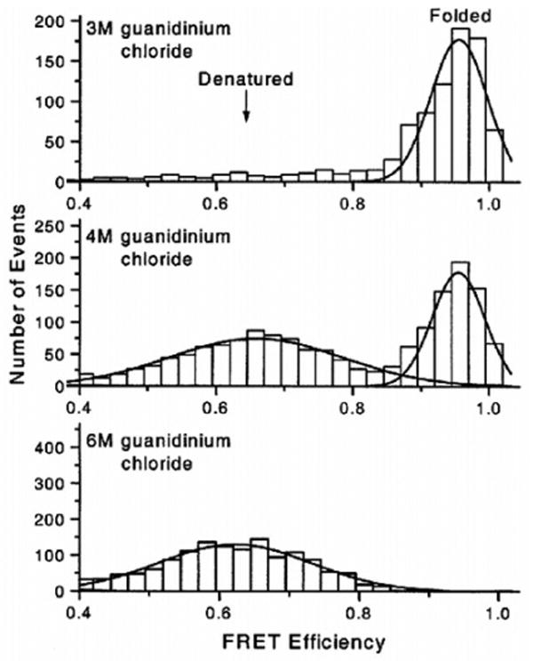
FRET efficiency distributions of CI2 at three different denaturant concentrations. Top, 3 M GdmCl (native conditions); middle, 4 M GdmCl (close to the midpoint of unfolding); and bottom, 6 M GdmCl (strongly denaturing conditions). The bimodal distribution of the FRET efficiency clearly indicates the two-state nature of the unfolding process. Adapted with permission from ref 110. Copyright 2000 National Academy of Sciences U.S.A.

4.1.2. Cold Shock Protein (Csp)

Csp is a 66 residue single-domain protein from the hyperthermophilic bacterium Thermotoga maritime, and like CI2, it obeys apparent two-state folding at the ensemble level.^63,161,162 Unfolding of Csp was monitored in a confocal microscope using freely diffusing molecules in solution. Labeling of Csp was accomplished by introducing two complementary fluorophores at two engineered cysteine (Cys) residues at the N and C terminus (wild-type Csp is devoid of Cys) using the sequential labeling method pioneered by Haas and co-workers.¹⁶³ Although the size of the polypeptide is (in principle) not a limiting factor, this method usually results in sample heterogeneity, unless the D/A- and the dye-permutated A/D-labeled analogues can be chromatographically separated. Such mixtures can lead to unwanted sample heterogeneity, as the conjugated dyes can exert a positional-dependent perturbation of the energy landscape of the modified protein or exhibit photophysical properties dependent on the local environment.

Similarly to the two-state folder CI2 studied previously, bimodal distributions of FRET efficiencies were observed at denaturant concentrations where both the native and the unfolded protein coexist (Figure 9A). However, when compared to CI2, the denatured subpopulation of Csp showed a much more pronounced shift in the mean FRET efficiency upon increasing the denaturant concentration (Figure 9B), which was again attributed to a hydrophobic chain collapse. The extent of chain collapse in Csp is perhaps surprising. For example, stopped-flow small-angle X-ray scattering (SAXS) provided little evidence for chain collapse preceding the rate-limiting barrier crossing event in protein L, ubiquitin, and acylphosphatase,^164,165 proteins that are comparable in size to Csp. These observations imply that the radius of the denatured state of these proteins does not change with denaturant concentration. Moreover, Kohn et al. employed SAXS and showed that the dimensions of most chemically denatured proteins employed for protein folding studies scale with polypeptide length according to the power–law relationship expected for random coil behavior. It has therefore been argued that the extensive chain collapse observed in Csp may be artifactual, due to stacking of the bulky, aromatic fluorophores under conditions where the protein is unfolded.¹⁶⁵ Although such a claim cannot be refuted completely with the available data reported by Schuler et al., fluorescence anisotropy control experiments ensured that the dyes are rotationally free over the donor fluorescence lifetime time scale. In addition, chain collapse in Csp was also detected with unlabeled Csp using the quenching of the triplet state of a single tryptophan by a cysteine in the same polypeptide chain.⁷³ Interesting new information about intrachain dynamics in denatured Csp could be obtained by comparing the width of the FRET efficiency distributions of denatured Csp with the distributions obtained from a conformationally rigid type II polyproline helix^89,166,167 labeled with the identical FRET–dye pair (Figure 9A). Surprisingly, the widths of the FRET efficiency distributions were identical for the flexible, chemically denatured Csp and the rigid polyproline reference peptide under solvent conditions that match the mean FRET efficiencies. On the basis of these observations, it was argued that variations in the end-to-end distance in unfolded Csp do not contribute to the width of the E distribution of the denatured subpopulation beyond that predicted from shot noise. Such a result is expected if the reconfiguration rates between the various conformational states accessible to the denatured polypeptide chain are fast relative to the millisecond observation window of the experiment. This interpretation differs from previous speculations on CI2,¹¹⁰ where the larger than expected E distribution width was partly attributed to interdye distance fluctuations on a time scale comparable or slower than the observation time. On the basis of their results, Schuler et al. could estimate an upper bound for the reconfiguration time of denatured Csp of ∼25 μs. When combined with Kramers theory for the kinetics and the experimentally determined folding rates from ensemble stopped-flow kinetic studies (millisecond barrier-crossing rates), this value transforms into a lower bound of 4 k_BT for the free energy barrier of folding. As the free energy of activation includes both enthalpic and entropic terms, its absolute magnitude cannot be determined experimentally for processes that occur in solution. The exercise by Schuler et al. thus clearly shows that single-molecule experiments can provide otherwise inaccessible information about elementary properties of folding reactions and their associated dynamics, even under equilibrium conditions.

Figure 9.

Probing the equilibrium unfolding of Csp with freely diffusing molecules. (A) FRET efficiency histograms for Pro₆ (left), Pro₂₀ (middle), and Csp (right) at various concentrations of denaturant. Black curves represent best fits of the experimental data to log-normal or Gaussian functions. The dashed line reflects the contribution of shot noise to the width of the distribution. (B) Dependence of the means of the measured FRET efficiency of Csp. Upper full symbols are derived from the native subpopulations, while lower full symbols are calculated from the denatured subpopulation. Open symbols are the apparent FRET efficiencies measured in an ensemble FRET experiment. The shift in the mean E of the denatured subpopulation of Csp most likely reflects a collapse of the polypeptide chain upon transfer from a good solvent (high concentrations of denaturant) to a poor solvent (low concentrations of denaturant). No such shift is seen in the folded subpopulation or in the rigid polyproline distance rulers. Note that the width of the distribution of the rigid polyproline rulers is comparable to the width of the denatured subpopulation of Csp, suggesting that slow conformational fluctuations on a time scale comparable or slower than the experiment (<1 ms). Adapted with permission from Nature (http://www.nature.com), ref 70. Copyright 2002 Nature Publishing Group.

The logical next step in the quest to understand structure and dynamics in the denatured state of proteins will be a systematic variation of the position and sequence separation of the D/A–FRET pair employed, for example, by varying the position of two uniquely engineered Cys along the polypeptide sequence. The various mean E values will report on the extent and the structural distribution of compaction within a polypeptide chain and will serve as useful distance constraints in MD simulations.¹⁴⁷ Furthermore, the use of recently developed microfluidic mixing devices¹⁶⁸ to transiently populate denatured conformers will allow their detailed characterization under conditions not accessible by equilibrium experiments (e.g., strongly native conditions). Last, single-molecule experiments also show great promise to study downhill folding, as the absence of a significant activation barrier allows a continuous change in structure upon solvent or temperature tuning. This, in principle, should allow a FRET-based imaging of the complete sequence of structures that a folded protein undergoes during folding and unfolding.¹⁶⁹

4.1.3. Ribonuclease H (RNAse H)

RNAse H is the latest addition to the still limited set of simple two-state folding proteins studied at the single-molecule level. As for Csp, sequential labeling was employed to equip RNAse H with Alexa Fluor 546 and Alexa Fluor 647 fluorophores at two engineered cysteines, but in contrast to the burst spectroscopy studies discussed above, Nienhaus and colleagues opted for single-molecule experiments with immobilized protein.^170,171 To prevent unspecific surface adsorption of the immobilized protein previously seen in another study,^127,139 the authors used chemically designed, biotinylated surface coatings prepared by spin coating (Figure 10). The surface coatings were made of ultrathin networks of isocyanate-terminated “star-shaped” poly(ethylene oxide) (PEO) molecules, cross-linked at their ends via urea groups to minimize the intertwining of a denatured polypeptide chain with the PEO polymer. Immobilization of Alexa Fluor 546/Alexa Fluor 647-labeled and biotin-tagged RNAse H was accomplished using a biotin–streptavidin (SAv) sandwich technique. Immobilized proteins were localized in a confocal microscope setup, equipped with two separate detection channels for measurements of the emission in two spectral channels to enable FRET experiments. Unfolding of RNAse H on star polymer (SP)-derived layers was completely reversible, even after 50 consecutive cycles of complete denaturation in 6 M GdmCl and refolding (removal of the denaturant by buffer exchange), with only minimal loss of surface-deposited protein (Figure 11).¹⁷⁰ Control experiments on bovine serum albumin (BSA)-coated or linear PEO polymer surfaces, considered to be ideal surface coatings for studies with immobilized DNA or RNA,^83,123,172 were only partially reversible and hampered by substantial substrate loss (BSA coating) or were fully irreversible (linear PEO surface). Moreover, values for free energies of folding and unfolding cooperativity (or m value), a constant proportional to the change in surface-accessible area upon unfolding calculated from surface-immobilized RNase H and experiments with freely diffusing molecules, agreed within experimental error and were significantly higher than control experiments with physisorbed molecules on BSA-coated glass slides, further demonstrating the resilience of the immobilized protein toward irreversible denaturation on the surface and the potential of single-molecule spectroscopy to quickly extract accurate thermodynamic parameters with only minute amounts of sample consumption.

Figure 10.

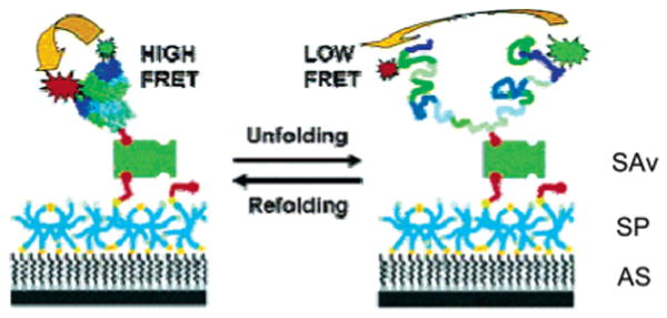
Schematic of protein immobilization on inert, biofunctionalized surfaces. Amino-silyated glass is coated with a layer of cross-linked six-arm SPs. Biotinylated and FRET pair-labeled RNAse H is added and coupled to the surface via biotin–SAv sandwich chemistry. Addition of denaturant destabilizes RNAse H, resulting in the population of denatured conformers. The interconversion between the folded and the denatured states can be followed using FRET between the donor and the acceptor fluorophores as a reaction coordinate. Adapted with permisison from ref 171. Copyright 2004 American Chemical Society.

Figure 11.

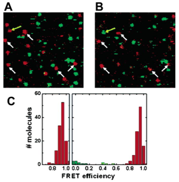
Confocal scans of a 10 μm × 10 μm sized area before (A) and after (B) 50 consecutive cyles of folding and unfolding. The white arrows indicate molecules that can be followed over many cycles. Out of >100 molecules, only four become trapped in a non-native conformation (one example is highlighted by a yellow arrow), demonstrating the high repellence of the polymer coating. (C) FRET histogram of >100 molecules before and after the folding–unfolding cycle. No increase in the width of the folded distribution is observable, ruling out structural heterogeneity induced by non-native interactions of the immobilized protein with the coated surface. Adapted with permission from ref 170. Copyright 2004 Wiley-VCH Verlag GmbH.

4.2. Application of μs-ALEX to Monitor Biomolecular Interactions and Folding

The ability for simultaneous monitoring of D–A distances and binding stoichiometries makes ALEX a promising tool for studying biomolecular interactions and folding. In a recent proof-of-principle experiment, the binding of D-labeled catabolite activator protein (CAP) to its cognate A-labeled DNA sequence was studied.¹¹¹ In the presence of cyclic AMP (cAMP), the affinity of CAP for DNA is extremely high and a large fraction of CAP was visualized as a complex with DNA, as inferred from D–A stoichiometry. The binding constant obtained from equilibrium titration of CAP with DNA (K_D ∼ 32 pM) was in excellent agreement with the literature value determined indirectly by a radioactive filter-binding assay. Future μs-ALEX experiments similar to those reported by Kapanidis et al. will allow detailed mechanistic studies of biological processes such as binding-induced folding of natively unfolded protein, the dissection of assembly pathways of large multicomponent complexes, and, of particular interest to the protein folding/misfolding problem, the visualization of template-directed oligomerization on a nucleating template (see also Figure 7 in ref 111).

In a first application of μs-ALEX to monitor protein-folding reactions, we studied the equilibrium unfolding of CI2, prepared from recombinant sources. The problem of site-specific labeling was solved by using a novel labeling strategy that involves high affinity protein interactions to selectively protect one of the two cysteines upon complex formation.¹⁷³ Figure 4C depicts representative 2D E–S histograms of D-only-labeled CI2, A-only-labeled CI2, and D/A-labeled CI2 at various concentrations of GdmCl. One-dimensional histograms of the stoichiometric ratio S (shown in blue color to the right of each histogram), obtained by projection of the entire 2D E–S histograms onto the vertical S-axis, show a unimodal S distribution with the expected mean S values ∼1 for the D-only sample, and ∼0 for the A-only sample. The S histogram of the D/A-labeled sample exhibits a major S peak at ∼0.5 and an additional minor peak at S ∼ 0. While the former peak arises from D/A-labeled molecules, the latter peak most likely results from A-only species due to incomplete D labeling. The D-only peak is completely absent in the sample without denaturant, but both D-only and A-only peaks increase substantially upon addition of 6 M GdmCl, probably due to buffer impurities and sensitized photobleaching due to denaturant–dye interactions. One-dimensional histograms of the FRET efficiency E for each sample are displayed on top of each 2D histogram (purple), obtained for doubly labeled species only (0.2 < S ratio < 0.6, selected area indicated by dashed purple box). The ability to digitally remove the D-only species that would otherwise contaminate the E histograms (particularly in the presence of high denaturant) will facilitate the study of proteins that unfolds via intermediates (resulting in broad E histograms in which D-only deconvolution may be difficult to achieve) or of large proteins, whose unfolding leads to a large distance separation of D and A dyes.

4.3. Protein Conformational Dynamics

Single-pair FRET experiments with freely diffusing molecules provide the most natural environment for water-soluble proteins and are completely free of surface artifacts. If the diffusing molecule fluctuates between different conformational states on a time scale much slower than the residence time of the molecule in the confocal spot, these conformational states will appear as static species (subpopulations) in E histograms. For two-state folders such as CI2 or Csp with folding rates in the millisecond range, only two subpopulations (native and denatured) are detectable. The short residence time of single molecules in the laser excitation volume puts a severe constraint on the time window in which dynamics within subpopulations can be studied (typically ∼1 ms), although new analysis methods presented above may address this problem soon. In principle, viscogenic solvents can be used to slow diffusion of biomolecules and increase their residence time in the focal spot, but such studies require careful control experiments to rule out unwanted changes of the folding energy landscape.^174,175 As demonstrated by Schuler et al.,⁷⁰ additional information about dynamics in subpopulations can be extracted from a careful analysis of the widths of E distributions, although this type of analysis is not without difficulties.¹³⁷ Even more detailed information about conformational dynamics is possible, if the continuous wave laser sources are replaced by pulsed lasers to enable TCSPC. Histograms of photon delay times can then be constructed and fitted to yield fluorescence lifetimes, which can then be used to extract distance distributions. Alternatively, immobilizing single molecules in agarose–, polyacrylamide–, or sol–gel matrices^126,176,177 or on supported polymer-treated surfaces (see above) can also dramatically increase the accessible time window, which is ultimately limited by the complex photophysics and photodestruction of the extrinsic organic fluorophores.

4.3.1. ns-ALEX

Distance fluctuations result in corresponding FRET fluctuations that can be studied by either ratiometric measurements of intensities or direct measurement of the donor fluorescence lifetime. The existence of different characteristics distances should therefore translate into multiple lifetimes. Because an accurate analysis of multiexponential fluorescence lifetime decay curves¹⁷⁸ is not possible from the limited number of photons emitted during a single-molecule burst, such analysis is performed with photons emitted from all bursts within a subpopulation (Figure 4C). Even though such lifetime decay curves could in principle be obtained from ensemble measurements, ns-ALEX offers two major advantages for this type of situation. First, ns-ALEX allows the elimination of the D-only subpopulation. D-only species may result from fluorophore bleaching, complex photophysics (nonfluorescent, long-lived triplet states), or incomplete labeling, as their presence can significantly bias E measurements at the ensemble level. Equally important, ns-ALEX can be employed in those cases where there are subpopulations that have overlapping properties that prevent them from being analyzed by ensemble methods, such as the unfolded state of proteins in the presence of a large fraction of folded molecules. In an ensemble experiment, this would result in a lifetime decay curve confounded by the presence of the fast donor decay due to the presence of the folded molecules. Recent ns-ALEX-based studies of ss DNA, dsDNA, and small proteins have revealed intriguing new results: (i) Short dsDNA, for instance, appears more flexible than expected from persistence length measurements on long dsDNA, and (ii) the electrostatic contribution to the persistence length of single-stranded poly-dT DNA varies as the power −1/2 of the ionic strength.¹⁰⁵ Third, studies on D/A-labeled CI2 (little residual structure under moderately denaturing conditions) and ACBP (highly collapsed) indicate that ns-ALEX is capable of differentiating between various extents of residual structure in the denatured subpopulation.

4.3.2. Single-Pair FRET Studies on Immobilized Proteins

Two immobilization formats have been used in the past to obtain dynamic information of the immobilized proteins and other biopolymers: direct, oriented, noncovalent adsorption of proteins on polymer-modified glass substrates,^31,127,139 and indirect immobilization of molecules by trapping in agarose gel¹²⁶ or vesicles.^138,179

Conformational Dynamics of Proteins and Enzyme Activities

Single-molecule studies on directly immobilized molecules were first reported on the staphylococcal nuclease (SNase).^118,180 This small 19 kDa Ca²⁺-dependent enzyme catalyzes the hydrolysis of DNA and RNA into mono- and dinucleotides. Labeling with a donor (TMR) was performed specifically on the unique cysteine (Cys²⁸) of the mutant, whereas labeling with the acceptor (Cy5) was performed nonspecifically on the protein's amines, with a yield of one donor–acceptor pair per molecule. The protein was engineered with a hexahistidine tag and fixed to a NTA-derivatized glass surface.¹¹⁸ Data acquisition was achieved in a two-channel confocal microscope with donor and acceptor fluorescence or donor s and p polarization time traces recorded simultaneously. Using 5 ms binning, Ha et al. reported E value fluctuations on time scales ranging from 10 ms to 1 s, which could not be accounted for by fluorophore reorientation or spectral shift. The typical time constant for this conformational fluctuations increased in the presence of a bound inhibitor (deoxythymidine diphosphate, pTp) indicating a reduced backbone flexibility in the presence of pTp. To study the activity of the bound enzymes, the authors then used a donor-only-labeled SNase and observed the binding and processing of 3′- or 5′-acceptor end-labeled 40 nucleotide ssDNA. From these experiments and control with an inactive SNase mutant still capable of binding ssDNA, they could observe a difference in dissociation times between the active and the inactive mutants, with the active mutants showing a shorter dissociation time with the 3′-ssDNA than with the 5′-ssDNA. These events could be interpreted as signatures of a processive 3′-to-5′ hydrolysis with the help of ensemble measurements testing for the enzyme processivity.

Chen et al. used a slightly more specific labeling approach to study the T4 lysosyme catalytic activity.^181,182 T4 lysozyme catalyzes the hydrolysis of polysaccharide chains of the Escherichia coli B cell wall matrix. The wild-type structure consists of two domains connected by an α-helix, which move as a hinge during conformational changes involved in the hydrolysis, as characterized by X-ray crystallography, NMR, and electron paramagnetic resonance. Two cysteines, among which one is partially buried and spatially restricted, were sequentially targeted by Texas Red maleimide and TMR iodoacetamide, taking advantage of the reactivity difference of maleimide and iodoacetamide with the buried cysteine. The crystallographic and MD data give distances of 30.5 and 35 Å between the cysteines in the closed and open states of the enzyme. The Förster radius of 50 Å calculated for the dye pair would result in these conditions in a donor intensity change of a factor 2–3, signature of the enzyme conformational change. Single enzymes attached to silanized surfaces using a bifunctional linker were observed by confocal microscopy after excitation of the donor (532 nm) and collection of the donor (D) and acceptor (A) fluorescence onto two APDs. Anticorrelated D and A fluctuations were observed over several seconds (independent of the excitation intensity), with (AFs) and CCFs characterized by a similar time constant of the order of 160 s⁻¹ at pH 7.2 and 80 s⁻¹ at pH 6 and saturating concentration of substrate, consistent with the reduced activity of the enzyme at lower pH. A large distribution of time constants was observed when a single time constant could be fit, suggesting static heterogeneity of the enzymatic activity. It was also observed that 10% of the molecules exhibited an additional slower component (1–22 s⁻¹) and 30% a faster one (∼500 s⁻¹), independent of the presence of substrate. The slower component could be attributed to local environment changes, whereas the faster one was tentatively attributed to spontaneous conformational fluctuations of the enzyme. Independent time-resolved experiments on Alexa Fluor 488-labeled T4 lysozyme showing similar time scale fluctuations could also suggest that these molecules were interacting with the surface.¹⁸³ Further analysis of individual donor time traces binned ever 0.65 ms showed fluctuations on the millisecond time scale characteristic of the enzymatic turnover and corresponding to hinge opening, substrate binding, and hinge closing, as verified by MD simulations. The open-time duration was observed to be Gaussian distributed within each single time trace, giving access to parameters of the hinge bending conformational dynamics energy landscape, in a simple model of 1D multistep random walk model in the presence of a force field. The final picture of T4 lysozyme enzymatic activity is thus one where (i) the time required for the enzyme to locate a binding site dominates the inhomogeneity in the overall reaction rate, (ii) subsequent steps have homogeneous rates among the individual enzymes examined, and (iii) multiple intermediate states are involved in the formation of the active enzyme–substrate complex.

Protein fluctuations may influence other important aspects of their function, in particular their binding affinity to other proteins or DNA. Several studies having dealt with calmodulin (CaM), a small calcium-signaling protein (148 amino acids), which is involved in diverse biological pathways, are illustrative of these aspects. ^184–186 The CaM conformational change upon Ca²⁺ binding was used by Tsien and collaborators to construct a double-fluorescent fusion protein for calcium sensing by FRET between the two fluorescent moieties¹⁸⁷ (Figure 12A). Dubbed “cameleon”, this construct includes a CaM-binding peptide domain of the myosin light chain kinase (73), which strongly interacts with CaM in the presence of Ca²⁺ ions on the four binding sites of CaM.¹⁸⁷ Brasselet et al. studied this molecule immobilized in agarose gel using dual-channel confocal microscopy. Donor and acceptor fluorescence time traces of a few seconds and with 20 ms resolution corresponding to individual CaM molecules were acquired at different calcium concentrations, from which average FRET efficiencies E were extracted and histogrammed (Figure 12B). The D–A distance obviously decreased at higher Ca²⁺ concentration, but the measured E distributions exhibited a larger width than that expected for shot noise-limited E histograms corresponding to the observed total signal (A + D):¹¹⁵

Figure 12.

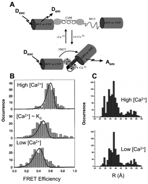
FRET study of CaM. (A) Schematic structures of the cameleon molecules used in ref 184. The GFPs are drawn as rigid cylinders, reflecting their crystal structures. Schematic structures of CaM without Ca²⁺, disordered unbound 73, and of the Ca²⁺–CaM–73 complex. (B) Histograms of Förster energy transfer efficiency, deduced from single-copy measurements of cameleon molecules for three different concentrations of calcium: Ca²⁺ saturation, intermediate concentration, and calcium-free agarose gel. The solid lines are the expected energy transfer efficiency distribution from the experimental noise, including shot noise and background noise as explained in the text. (C) Distributions of CaM donor–acceptor distances at high and low calcium levels using 75 μs bins. Bins containing donor or acceptor counts that were eight times above the standard deviation of the background signal, or six times above the standard deviation of the average sum of donor and acceptor counts, were included. (A) Adapted with permission from Nature (http://www.nature.com), ref 187. Copyright 1997 Nature Publishing Group. (B) Reprinted with permission from ref 184. Copyright 2000 American Chemical Society. (C) Adapted with permission from ref 185. Copyright 2004 American Chemical Society.

$$\sigma \left(E\right)=\sqrt{\frac{E\left(1-E\right)}{\text{A}+\text{D}}}$$ (20)

Suspecting some conformational dynamics at the origin of these large E distributions, the authors first eliminated orientational dynamics (the κ² factor of eq 8) as the origin of the observed width by performing single-molecule anisotropy measurements for the donor and acceptor fluorophores. Measuring the intratime trace E fluctuation ΔE by their root-mean-square, it appeared that those fluctuations could not be fully accounted for by shot noise. The very short duration of most time traces, however, did not permit to go beyond this analysis, and examination of CCFs and AFs of the signal for a couple of time traces hinting at a typical fluctuation time scale of ∼100 ms should probably be considered inconclusive. Slaughter et al. revisited this problem using a double cystein mutant of CaM, which was site-specifically labeled with a FRET pair.¹⁸⁵ Observations were done in solution using dual-color FCS using a single laser excitation (donor), and cross-correlation curves were obtained from 5 μs-binned time traces of diffusing molecules at various Ca²⁺ concentrations. The nondiffusive part of these curves was fitted with a sum of two exponential decays (similar to the last term of eq 19), yielding time constants in the 150–300 μs and 5–45 ms range for the diverse concentrations tested. Interestingly, at low (<40 nM) and high (100 μM) concentrations, quasi-identical values were recovered, whereas at intermediate concentration (1 μM), longer time constants were observed. To explore the nature of these fluctuations, E histograms of observed burst E values were converted in distance distributions and plotted (Figure 12C). Three populations were observed as follows: (i) a major, broad distribution centered around 38 Å; (ii) a minor, broad distribution around 55 Å; and (iii) a narrow distribution around 28 Å. The large distance corresponds to that predicted by the crystal structure for the Ca²⁺–CaM species, whereas the intermediate distance seems to correspond to the NMR structure of the Ca²⁺-free CaM. The short distance is similar to that reported by other ensemble methods but does not correspond to any known structure. In comparison with the previous study, which used a lower time resolution but immobilized molecules (and a slightly different system), this work revealed the presence of subpopulations of conformers, interconverting rapidly with the time scales reported earlier. The functionality of these fluctuations remains, however, unclear as this work did not involve any CaM ligand. A recent study using a single-molecule fluorescence quenching technique and a Nile Red dye-labeled peptide ligand¹⁸⁶ has however confirmed that such fluctuations directly affect the binding properties, recovering a dependence of the fluctuation time scales on calcium concentration.

Protein Folding

Hochstrasser and collaborators used a single-molecule FRET-based approach to report the first study of protein folding.^127,139 The model system used was the DNA-binding domain (a cooperatively folded coiled coil dimer) of GCN4, a transcription factor from yeast. Labeling was facilitated by the dimeric architecture of the domain. Each coil subunit was synthesized independently using solid phase chemistry. The N termini were selectively deprotected and reacted with TMR and Texas Red as donor and acceptor fluorophores, respectively. The singly labeled subunits were assembled into the coiled-coil and, to prevent chain dissociation, chemically cross-linked via a disulfide bond formed between two cysteines close to the C-termini of each subunit. Immobilization of labeled, disulfide cross-linked GCN4 was achieved via electrostatic interaction between an aminosilanized glass surface and a negatively charged pentaglutamate sequence added to the two C-termini. The initial folding trajectories reported by Jia et al. exhibited exceptionally well-resolved, anticorrelated fluctuations in D and A emission intensity, which was taken as evidence for folding–unfolding cycles of the immobilized protein. In a more detailed study, auto- and cross-correlation analysis of the calculated FRET efficiency time traces at various denaturant concentrations revealed fluctuations within immobilized GCN4 with characteristic time scales in the order of 1–100 ms,¹³⁹ in good agreement with bulk solution data. Unfortunately, however, the E histograms obtained by analysis of the folding trajectories with immobilized GCN4 were significantly broader than those obtained from control experiments performed with freely diffusing molecules. The discrepancy was particularly strong under conditions where the immobilized protein is predominantly unfolded, pointing out the possibility of strong non-native interactions between the immobilized protein and the glass surface that may complicate a rigorous interpretation of the experimental data.

To minimize a possible surface-induced perturbation of the free energy landscape of the immobilized protein, Boukobza et al. encapsulated TMR-labeled BSA and Texas Red-labeled AK in lipid vesicles, doped with a small quantity of biotinylated lipid for subsequent surface deposition on a biotinylated, glass-supported lipid bilayer using streptavidin–biotin sandwich chemistry (Figure 13A). Unilamellar vesicles with an average diameter of 100 nm, much larger than the diameter of the trapped molecule but smaller than the diffraction-limited excitation spot, were prepared by rehydration of thin films of dried lipid with a buffer solution containing appropriate amounts of labeled protein and denaturant, followed by repeated extrusion through a membrane. The number of trapped molecules per vesicles was determined from long fluorescence time traces, exploiting the sudden, stepwise bleaching of single chromophores. The number of trapped molecules followed a Poisson distribution, with an average occupancy of 0.65 molecules per vesicle. Polarization distributions obtained with vesicles loaded with a single-labeled molecule resembled that of freely diffusing molecules and were much narrower than control experiments with molecules directly deposited on untreated glass surfaces, ruling out a significant perturbation of the free energy landscape of the trapped molecule due to confinement or non-native interactions with the negatively charged vesicle interior.

Figure 13.

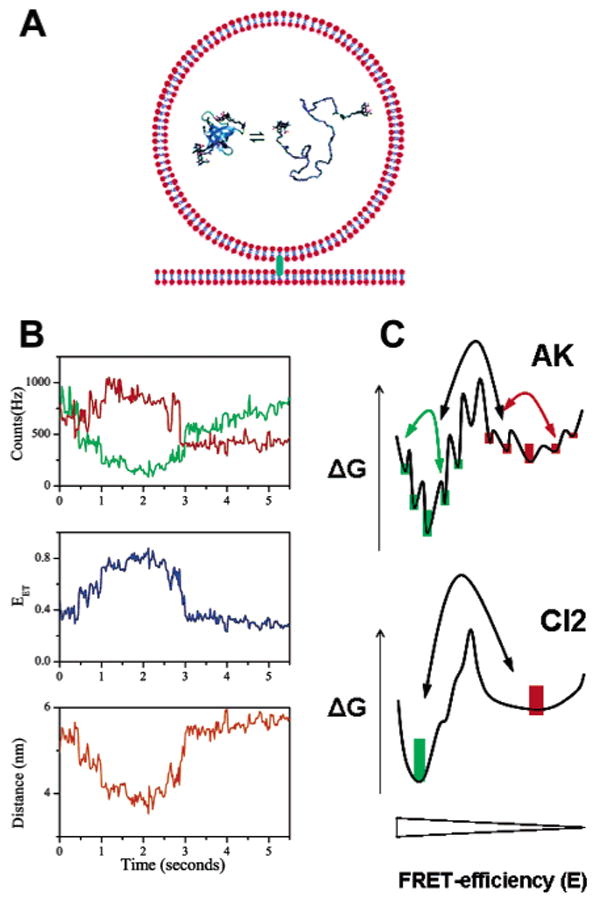
Probing conformational dynamics within single, surface-immobilized molecules. (A) Encapsulation of single molecules in lipid vesicles. Immobilization of the trapped molecule is achieved indirectly by tethering the biotinylated vesicle to a streptavidin-coated polymer coating. As the diameter of the encapsulating vesicle (∼100 nm) is considerably larger than the diameter of the trapped molecule, the trapped molecule can diffuse freely, thus minimizing a perturbation of the energy landscape due to confinement and nonproductive interactions of the trapped protein with the vesicle interior. (B) Representative single-molecule folding trajectories of encapsulated AK at denaturant concentrations around the midpoint of unfolding, conditions at which the native and denatured subpopulations are equally populated. The top panel shows time traces of the D and A emission (green and red, respectively), employing 20 ms bin times. D and A emission are anticorrelated, indicative of conformational transitions within the polypeptide. Notice, however, that the D emission continues to increase after bleaching of the acceptor (t ∼ 3 s), suggesting a variable environment (e.g., diffusion within the vesicle). Two types of fluctuations are visible in the E trajectory: fast, stepwise fluctuations that cannot be resolved and slow, continuous transitions that can take >1 s for completion. The middle panel depicts a FRET efficiency trajectory calculated from the signals in the top panel, whereas the interprobe distance trajectory (calculated according to Förster theory) is shown in the bottom panel. (C) Schematic of a 1D energy landscape for AK and CI2 at denaturant concentrations close to the midpoint of folding, obtained by averaging of the folding landscape over many degrees of freedom and projection onto the FRET efficiency axis. Both energy landscapes exhibit two global free energy minima separated by a free energy barrier, as suggested by the bimodal FRET efficiency distributions. The landscape of AK is characterized by local free energy barriers and traps, resulting in fluorescence time trajectories that can start and end at any FRET efficiency value (the population weight of the folded species is indicated by green bars, while the unfolded conformers are color-coded red). The landscape of CI2 is smoother, and time trajectories exhibit fluctuation between two relatively constant levels of FRET efficiencies. (A) Adapted with permission from ref 188. Copyright 2004 American Chemical Society. (B) Adapted with permission from ref 138. Copyright 2003 National Academy of Sciences USA.

Using vesicle encapsulation, Rhoades et al.¹³⁸ first reported detailed information about conformational dynamics of the 214 residue protein AK. Fluorescence emission from AK-loaded vesicles located on the bilayer surface with a stage-scanning confocal microscope was split into donor and acceptor channels. After correction for D-only leakage into the A channel, the signal was represented as 20 ms resolution time traces. At denaturant concentrations where native and unfolded AKs are equally stable, the distributions of FRET efficiencies calculated from such folding trajectories were bimodal, suggesting two major subpopulations separated by an energy barrier, an observation that was not expected from the non two-state folding behavior of AK at the ensemble level. The mean E of the low-FRET subpopulation was higher than the corresponding value of the denatured subpopulation under strongly denaturing conditions, whereas the mean E of the folded subpopulation was shifted to lower values as compared to the reference in the absence of denaturant. While the increase in the mean E of the denatured subpopulation upon transfer from high concentrations to intermediate concentrations of denaturant can be explained by polypeptide chain collapse, the relatively large decrease in mean E of the folded subpopulation, which was not detectable in previous solution-based studies on CI2⁹¹ or Csp⁷⁰ needed a new explanation. The authors favored a model in which the native state is in rapid equilibrium (interconversion rates much faster than the observation window) with partially open conformations, explaining the increased width of the native subpopulation under these conditions. Perhaps most interesting was the observation that the amplitudes of the transitions in the folding trajectories showed a wide distribution, with a preference for small steps starting and ending at any E value, indicative of a rugged energy landscape with two global free energy minima (as indicated by the bimodal E distribution) and numerous local energy barriers within each of the two global minima (Figure 13C). Two types of folding transitions were detectable (Figure 13B): (i) Some folding trajectories exhibited sudden jumps in E that could not be resolved with the time-resolution of the experimental setup, as well as (ii) slow transitions, in which E changes gradually over a time scale of up to >1 s. While the former are characteristic of stochastic barrier-limited enthalpic transitions between different conformational states, the molecular origin for the slow transitions remains elusive. Possible explanations mentioned by the authors include (i) a decrease in intrachain diffusion experienced by the protein in certain regions of the energy landscape, resulting from directed motion on the energy landscape slowed by multiple local traps, (ii) the formation and dissolution of a folding nucleus required to overcome local energy barriers, or (iii) barrier-crossing events rate-limited by entropy.

In a subsequent study, Rhoades et al.¹⁸⁸ performed similar experiments with the two-state folder Csp at denaturant concentrations close to the midpoint of unfolding. Time trajectories of FRET efficiency were less complex than that obtained with the multistate folder AK and showed a rather narrow distribution of transition sizes, indicative of a smooth landscape with little local ruggedness (Figure 13C). The FRET efficiency cycled between levels of high FRET (mean E ∼ 0.8) and low FRET (mean E ∼ 0.2) values that agreed reasonably well with those obtained in a previous solution experiment.⁷⁰ Transitions between the two FRET levels occurred within the time-resolution of the experiment, even if much shorter integration times (100 μs) were used, and only an upper limit estimate of ∼200 μs could be given for the barrier transit time (the time that the molecule spends crossing the barrier). Nevertheless, this upper limit estimate is consistent with the lower limit for the reconfiguration time in the denatured obtained from burst experiments in solution.⁷⁰ Histograms of the residence time (the time that a molecule stays in one of the two FRET states before the next transition) were constructed and could be fitted with a single exponential. The rate constant obtained from the histogram fit (0.62 s⁻¹) agreed reasonably well with the rate obtained from stopped-flow fluorescence bulk experiments under identical conditions (0.39 s⁻¹),⁷⁰ further reinforcing the two-state folding of Csp.

Taken together, the two initial studies by Rhoades et al. show that single-molecule studies with surface-immobilized molecules provide unique information about the free energy landscapes of proteins, which is not readily visible in solution experiments. More experiments on other model systems are needed, however, to show how representative the results obtained with AK are for complex folders, to benchmark the different folding scenarios predicted by the funnel theory, and to extract both local and global characteristics of these folding energy landscapes. The next logical step will be the extension of the method to include proteins that obey a three-state folding mechanism at the ensemble level.^52,53 The question here is whether folding intermediates are productive on-pathway conformers or off-pathway traps.⁵⁵ An unambiguous answer is difficult to obtain from kinetic or native-state hydrogen-exchange experiments at the ensemble level, as the vast majority of intermediates for which thermodynamic and kinetic information that is available can be fitted equally well to both on-pathway and off-pathway kinetic schemes.⁵² However, such a distinction is straightforward at the single-molecule level, provided that the intermediate is spectroscopically distinguishable from the denatured and native conformers and populated sufficiently long to accumulate enough photons for its detection. If an intermediate is off-pathway, it must unfold before folding in the native state can occur, and folding trajectories will exhibit transition to the high-FRET state only directly from the denatured state. On the contrary, if an intermediate is obligatory, the native state can never be reached directly from the low-FRET state and always occurs via a state with intermediate FRET. That such studies on proteins should be possible has been recently demonstrated by Zhuang et al., who studied the Mg²⁺-induced folding of the tetrahymena ribozyme. Their results indicate at least three distinct folding pathways, designated as “fast”, “slow”, and “misfolding” pathways. The fast pathway was totally hidden at the ensemble level.

4.4. Probing Biomolecular Dynamics Via Fluorescence Quenching and ET

Fluorescence quenching designates a decrease in fluorescence emission intensity due to the apparition of a nonradiative decay channel from the excited state (see Figure 1 and accompanying text). Quite a diverse set of phenomena can result in fluorescence quenching. We have abundantly discussed FRET, which can be viewed also as quenching of the donor fluorophore, although it is more useful to look at it as an anticorrelated change in fluorescence emission of the donor and acceptor fluorophore. This allows ratiometric measurement to be performed (measurement of the FRET efficiency E), canceling out the effect of a varying excitation intensity, which is especially relevant for diffusion measurements.^91,115 In other cases of quenching, however, there is no other signal to monitor than the fluorescence intensity (or spectrum, lifetime, or polarization) of a single type of fluorophore. Some examples are (i) FRET with a nonfluorescent acceptor molecule such as Dabcyl,¹⁸⁹ (ii) quenching by a nearby residue, (iii) self-quenching of two identical fluorophores,^190,191 (iv) enzymatic modification of a fluorophore,¹²⁶ and finally (v) ET to (or from) a built-in electron acceptor (or donor).^31,94

Except for the case of a nonfluorescent acceptor, the impossibility to perform ratiometric measurement is offset by the advantage of not having to label the molecule of interest with more than one dye (or possibly none at all if the biomolecule is naturally fluorescent) and the simplicity of the detection path design. We will review here several cases where this approach has been used very successfully, putting a special emphasis on ET.

4.4.1. Quenching by a Nearby Residue

Kästner et al. used quenching by the protein itself to study citrate binding to single cystein mutants of the K. pneumoniae Na⁺-dependent citrate carrier (CitS) transmembrane protein labeled with a single dye (Alexa Fluor 546 or Alexa Fluor 568).¹⁹² The proteins were immobilized on Ni–NTA-treated surfaces via an N-terminal His-tag and visualized using a stage-scanning confocal setup. Only one mutant kept its activity after labeling, corresponding to an intracytoplasmic site of attachment for the fluorophore. Upon addition of citrate at a saturating concentration for the extracellular binding site, but well below the binding constant for the intracellular site (locus of release of citrate after membrane transport), a decrease in fluorescence was observed. The quenching of the dye fluorescence was due to a conformal rearrangement of the protein bringing the fluorophore in close proximity with an aromatic residue. Although of modest impact, this study shows that a rather simple labeling strategy can be efficiently used to study conformational changes in a protein.

4.4.2. Self-Quenching of Identical Fluorophores

Zhuang et al. first introduced this method to study the folding of titin, a large protein comprised of 200–300 modules of immunoglobulin type C2- and fibronectin type III-like domains connected by unique peptide sequences.¹⁹⁰ Labeling of 85% of the cystein residues with Oregon Green 488 did not modify the folding properties of the protein, as verified by single-molecule force spectroscopy on molecules adsorbed on a gold surface, using an atomic force microscope.¹⁹³ A sawtooth pattern with periodicity of ∼25 nm was observed as expected in the force vs extension curves for 40% of the labeled titin molecules, matching that observed for the same proportion of unlabeled proteins. These features disappeared in the presence of a denaturing solution (8 M GdmCl) but reappeared after removal of the denaturant. This reversibility of GdmCl-based denaturation was at the basis of the fluorescence experiments performed on labeled titin molecules adsorbed on a glass surface. To avoid nonspecific denaturation of the protein by contact with the surface, the authors used a high-density surface coverage, with only a minute proportion of labeled proteins (1%). Upon addition of denaturant, the fluorescence of individual molecules monitored with a scanning-stage confocal microscope increased progressively, up to 3.9-fold upon complete denaturation. Because this reversible increase was reduced when lower labeling efficiencies were used, the authors concluded that the increase was due to a suppression of self-quenching of the dyes upon spatial separation due to denaturation of the protein. Using rapid buffer exchange (with a dead-time of ∼10 ms), they could rapidly modify the protein environment from native to denaturing and observe a corresponding fluorescence increase and decrease on individual molecule time traces. These were interpreted as due to the unfolding and refolding of titin, respectively. An average 20 ms was necessary to unfold the protein, whereas a broad distribution centered around 32 ms was measured for the refolding time. Although the precise nature of the unfolding kinetics or the reason for the dispersion in refolding time (different pathways, local environment) could not be elucidated, the origin of the self-quenching could be demonstrated and attributed to interaction between fluorophores attached to the same domain, opening the possibility to use this approach in single-domain proteins. These results were, however, put in perspective by a subsequent report by Grama et al., who performed similar experiments using TMR instead of Oregon Green 488.¹⁹¹ They observed a similar phenomenon, except for time constants for the increase and decrease of fluorescence an order of magnitude larger than previously found (0.51 and 0.73 s, respectively). They could attribute this fluorescence variation to self-quenching of TMR but also show that the kinetic signature was that of the dissociation of dye dimers, a phenomenon that was verified by direct measurement of unquenching on highly concentrated solutions of dyes only. More revealing was the measurement at the ensemble level of tryptophan fluorescence in titin molecules, which showed a biexponential unfolding kinetics with time constants of 27 and 234 s. To explain these discrepancies, the authors verified that the fluorescence of TMR was insensitive to low pH conditions, which are on the other hand known to trigger unfolding in proteins. The addition of HCl to labeled titin molecules resulted in their denaturation but no increase of the TMR fluorescence, indicating that the dye dimers had not been perturbed by the acid denaturation of the protein. Addition of GdmCl resulted in an increase of fluorescence, as observed before. In conclusion, these experiments could indicate that folded and unfolded titin molecules both bring the dyes in close proximity, although their structures are extremely different. Undeniably, this single-molecule strategy, which seems the only one adapted to large proteins, can result in relatively ambiguous results.

Frieden and collaborators have used self-quenching in conjunction with FCS to study a simpler protein (131 amino acids) in its denatured state, the intestinal fatty acid-binding protein (IFABP).¹⁹⁴ In its native state, IFABP consists of two β-sheets enclosing a cavity in which the fatty acid binds. Indications of transient residual structure in the unfolded state motivated the authors to design an approach that would allow monitoring of the kinetics of interconversion, if not the conformations themselves. As no structural information was sought, the use of quenching was a natural option and was used in this case, by labeling a double cystein mutant with TMR (one Cys in each β-sheet). In the presence of 2 M GdmCl, the protein fluorescence is markedly quenched in comparison with labeled single mutants, suggesting transient encounters of the two fluorophores in the unfolded state. To study the dynamics of these conformational fluctuations, FCS of the TMR signal was used. For single TMR labeling, the FCS curve could be well fit by eq 18, with a diffusion time τ_D = 180 μs, whereas the doubly labeled sample resulted in a FCS curve exhibiting two characteristics times, as described by eq 19, with a comparable diffusion time τ_D = 193 μs and a relaxation time τ_R = 1.8 μs at 2 M GdmCl and 1.6 μs at 3 M GdmCl. Because these values of τ_R did not depend on the excitation power but increased linearly with increasing viscosity of the solvent, it was concluded that they were characteristic of a diffusive process. The relative amplitude A of this dynamics (eq 19) followed the same sigmoidal dependence as the steady-state fluorescence signal with respect to GdmCl concentration, indicating that the signal is indeed a signature of dye–dye interaction (and thus protein conformational fluctuations) appearing upon denaturation of the protein in a similar cooperative way. Using acidic pH denaturation, which is thought to result in a molten globule conformation keeping some residual secondary structure, the FCS curves could be fitted with eq 19 but with larger values of τ_R (τ_R = 2.5 μs at pH 2). The addition of 100 mM KCl increased this value even further (τ_R = 8 μs), indicating a reduction of the frequency of these fluctuations, in agreement with far UV circular dichroism experiments showing that in these conditions, the denatured protein has more structure and a spectrum resembling that of the native protein. In conclusion, although the nature of the conformational fluctuations could not be elucidated (which would need more mutants), this rather simple approach shows its potential utility to address questions about the limiting kinetic steps in the folding and unfolding process.

4.4.3. Quenching Due to Enzymatic Activity

In a very elegant experiment, Lu et al. studied the activity of single cholesterol oxidase enzymes (COx) from Brevibacterium sp., a flavoenzyme that catalyzes the oxidation of cholesterol by oxygen.¹²⁶ The active site of the enzyme (E) comprises a flavin adenine dinucleotide (FAD) moiety, which is naturally fluorescent when oxidized but is not when reduced. During the catalysis, FAD is first reduced by a cholesterol molecule to FADH₂ and then oxidized by O₂, yielding H₂O₂. By confining the molecules in a 1% agarose gel, stage-scanning confocal images of the FAD fluorescence could be obtained, and time traces of the intensity of individual enzymes were acquired sequentially for minutes, due to the protection of the fluorescent FAD moiety by the rest of the protein. In the absence of cholesterol, the only noticeable features were bleaching events, whereas in the presence of cholesterol and oxygen in saturating concentrations, the fluorescence appeared intermittent, independently from the excitation intensity, excluding a photoinduced origin to this phenomenon. This intermittent behavior was directly related to individual events of enzyme reduction (switching off) and enzyme oxidation (switching on) by studying the distribution of on- and off-times. Both were distributed as a convolution of two exponentials as expected for a two-step reaction of the form:

$$\text{E}-\text{FAD}+\text{S}\stackrel{k_1}{\to }\text{E}-\text{FAD}·\text{S}\stackrel{k_2}{\to }\text{E}-{\text{FADH}}_2+\text{P}$$ (21)

for the reduction reaction where S is the enzyme substrate (cholesterol) and P its product and a similar one for the oxidation reaction. Rate k₁ increased proportionally to the cholesterol concentration, further confirming this Michaelis–Menten reaction mechanism. Lu et al. next explored the values of k₂ measured from different enzymes using 5-pre-gene-3β-20α-diol substrate (a derivative of cholesterol with a longer waiting time before oxidation, which renders k₂ rate-limiting). Their result showed a very broad distribution of average rates, indicative of static heterogeneity in the rate values. Pushing the analysis further, they explored the AF of the fluorescence intensity of single enzymes observed in rate-limiting conditions where the reaction reads

$$\text{E}-\text{FAD}\underset{k_2\prime }{\overset{k_2}{\rightleftarrows }}\text{E}-{\text{FADH}}_2$$ (22)

The AF is expected to decrease exponentially with a decay rate k₂ + k₂′ but instead was observed to not obey this simple law, possibly indicative of variations (dynamic disorder) of the rate constants. This was confirmed by the existence of strong memory effects for the on-times on a short time scale (over a few seconds), further quantified by simulations of a simple reaction pathway involving two interconverting conformers of the enzyme, each characterized by a different k₂ rate. Although the nature of these hypothetical conformers could not be determined, their signature could be documented by measuring individual enzyme spectra over time. Further analysis using higher order correlation functions did not help discrimination between this simple model involving two alternative conformations and another involving a continuum of conformers.¹⁹⁵ This seminal study definitely confirmed the existence of static and dynamic heterogeneity in enzymes,^196,197 illustrating the power of single-molecule fluorescence studies for elucidating enzymatic reaction mechanisms inaccessible via ensemble methods.

Other enzymes have been studied using a similar approach. The activity of horseradish peroxidase (HRP) was investigated by Rigler and collaborators using FCS on immobilized molecules.^198,199 Oxidation of the nonfluorescent dye dihydrorhodamine 6G by HRP in the presence of H₂O₂ leads to two fluorescent Rhodamine 6G molecules per enzyme cycle, each oxidation cycle consisting in the binding of the substrate, oxidation, and product release:

$$\text{E}+\text{S}\underset{k_{\text{D}}}{\overset{k_{\text{A}}}{\rightleftarrows }}\text{ES}\stackrel{k_{\text{O}}}{\to }\text{EP}\ast \stackrel{k_{\text{R}}}{\to }\text{E}+\text{P}$$ (23)

where the asterisk indicates the only visible species (free products are released and diffuse away). For all practical purposes, the authors modeled the system as a two-state model, with one invisible species (E) and one visible one (EP), interconverting as:

$$\text{E}\underset{k_{-1}}{\overset{k_1}{\rightleftarrows }}\text{EP}\ast$$ (24)

with effective rates k₁ and k₋₁. Fluctuating levels of fluorescence were detected by confocal microscopy, one molecule at a time, and series of fluorescence AFs were recorded every 10 s. These AFs exhibited a noticeable variability for each enzyme, which the authors attributed to variability in k₁ only, due the many processes leading to the fluorescent species EP*. In addition, individual or averaged AFs for a single molecule could not be fitted with eq 19 (assuming τ_D = ∞) and required an additional stretched exponential component, attributed to the distribution of rates k₁.¹⁹⁸ To investigate the possible origin of this dispersion, Edman and Rigler looked at higher order correlation functions to compute a measure of the non-Markovian character of the dynamics (existence of memory effect), the non-Markovian function (NMF):¹⁹⁹

$$\text{NMF}({\tau }_1,{\tau }_2)\propto \frac{G({\tau }_1,{\tau }_2)}{G({\tau }_2)}-G({\tau }_1)$$ (25)

where G(τ₁,τ₂) is the two-point intensity correlation function:

$$G({\tau }_1,{\tau }_2)=\frac{\langle I(t)I(t+{\tau }_1)I(t+{\tau }_1+{\tau }_2)\rangle }{\langle I(t)\rangle \langle I(t+{\tau }_1)\rangle \langle I(t+{\tau }_1+{\tau }_2)\rangle }$$ (26)

For a Markovian process in which the probability P(E_N|E_N−1) to be in a particular state E_N in the next step N when the system is in the current state E_N−1 does not depend on the past trajectory, the following relations hold for the probability: P(E_N|E_N−1; E_N−2) = P(E_N|E_N−1), and the NMF is uniformly zero. Departure from this behavior is a strong indication of a non-Markovian behavior, which is precisely what was observed for individual HRP as shown in Figure 14C. This led the authors to suggest a reaction scheme for HRP in which the enzyme goes through a number of intermediate configurational states before oxidation of the substrate (Figure 14A), in opposition to a dynamic disorder due to multiple active conformers, each characterized by a different kinetic constant k₁ (Figure 14B).

Figure 14.

Single-molecule spectroscopy of HRP. Descriptions of two possible origins of the stretched exponential kinetics in the one-time autocorrelation of the fluorescence intensity observed in individual HRP enzymes. In part A, there are a number of intermediate states (E_k, k = 1,2,3,…,n) that the enzyme may traverse before a new product is formed (EP*). In part B, transitions to the EP state are exponential for each substrate turnover; however, each turnover may occur via any of the n channels, each with a different state transition probability. (C) Typical memory landscape NMF-(τ₁,τ₂) of a molecule observed for 110 s, showing that scheme A is appropriate for the description of the observed dynamic disorder in HRP. Adapted with permission from ref 199. Copyright 2000 National Academy of Sciences U.S.A.

Flomebom et al. recently presented yet another analysis of dynamic disorder in enzymes by studying the activity of lipase B from Candida antarctica (CALB).^200,201 Lipase B catalyzes the hydrolysis of esters and generates bursts of fluorescence when a nonfluorogenic ester of carboxyfluorescein is provided as a substrate. Individual enzymes nonspecifically adsorbed on hydrophobic surfaces were monitored over tens of minutes using confocal microscopy. Intermittent fluorescence emission was analyzed as described by Lu et al.¹²⁶ The first result was an exponentially decaying distribution of on-times, corresponding to a fixed dissociation rate of the fluorescent product from the enzyme (k⁻¹ ∼ 1 ms). Off-times, on the other hand, were distributed as a stretched exponential:

$$P_{\text{off}}(t)\propto exp[-{(t/{\tau }_0)}^b]$$ (27)

where τ₀ = 1.15 μs and b = 0.15 for various substrate concentrations. A closer look at the temporal distribution of the off durations revealed a phenomenon of “bunching”, i.e., a memory effect (Figure 15A). Flomenbom et al. considered a reaction scheme analogous to that described in Figure 14B but where each different conformation E_N is interconnected to nearby ones in configurational space (Figure 15B). Analysis of the data within this theoretical framework resulted in a description where the enzyme is characterized by a broad distribution of reaction rates exhibiting a peak 〈 k 〉_fast⁻¹ ∼ 8 ms and a power law decay. Conformers were found to interconvert with a typical rate 〈 γ 〉_fast→slow⁻¹ ∼ 45 ms.

Figure 15.

CALB enzyme activity. (A) The trajectory of the time durations of the off-state events as a function of chronological event index for a substrate concentration of 1.4 μM. Noticeable along this trajectory are groups of successive fast events (each event in the group has an off value of <35 ms). (B) The fluctuating enzyme model. The off state consists of a spectrum of N-coupled substates (circles). Also indicated are the coupling rates between the conformations and the enzymatic reaction rates. Squares indicate the on states. Reprinted with permission from ref 201. Copyright 2005 National Academy of Sciences U.S.A.

These different enzymes (Cox, HRP, and CALB) have thus turned out to be all characterized by dynamic disorder, information that only single-molecule spectroscopy could provide. Although the activity of these surface-bound enzymes was compared to the bulk activity, it still remains possible that some unsuspected surface interactions may be partly responsible for the observed disorder. More sophisticated experimental methods, for instance measuring the time-resolved polarization anisotropy of an attached dye,^183,202 could possibly remove this ambiguity. The different methods developed to analyze the observed kinetics in terms of different interconverting active or inactive conformers, with or without variable catalytic activity, will certainly motivate more sophisticated studies to further refine our picture of single-enzyme function.

4.4.4. ET

ET between a fluorescent donor or acceptor moiety and an electron acceptor/donor happens at distances comparable to the regime of self-quenching discussed previously (<2 nm), thus at much shorter distances than those characteristic of FRET (4–8 nm). As it reports on very close interactions, it is a tool complementary to FRET and has been used in particular to study fast fluctuations of small amplitude. However, ET does not require precise molecular contact and the existence of diverse possible mechanisms of transfer (through space or via superexchange mechanisms⁹²) requires a thorough characterization of each system before inference on distance fluctuations can be made. Experimentally, ET is detected by a reduction in fluorescence emission (quenching) of the fluorophore,²⁰³ as well as a reduction of its lifetime.^204,205

Polypeptides

Sauer and collaborators have studied PET to red oxazine dyes (MR121, τ = 1.85 ns) from guanosine residues in DNA oligonucleotides²⁰⁶ or tryptophan residues (Trp) in polypeptides⁹⁴ at the single-molecule level. In these systems, quenching was shown to require almost van der Waals contact by ensemble measurement of bimolecular quenching constants, thus validating the use of ET to monitor close contact formation between the dye and the quencher. Neuweiler et al. studied two short peptides (15 and 20 amino acids, respectively, with a single internal Trp) derived from the transactivation domain of p53, which is targeted by several proteins⁹⁴ (Figure 16). By exciting the dye with a continuous wave laser, the authors did not rely on fluorescence lifetime measurements, which only gives access to subnanosecond phenomena, but instead measured interval distribution between successive photons on a 5 μs time scale with nanosecond resolution (Figure 16B).⁹⁴ Measuring the photon distance distribution (PDD) is equivalent to measuring the AF of the fluorescence at time scale where there is zero probability to have emission of an intermediate photon. On this time scale, excitation, relaxation to the ground state, and quenching by ET are instantaneous, and the kinetic scheme comprises only association and dissociation with the quenching tryptophan residue in the ground state or triplet state. Introducing a contact formation rate k₊ and two dissociation rates and k₋ and k_Ph*, the kinetic equations corresponding to Figure 16A can be solved, resulting in a multiexponential decay for the AF. Separate measurement of the triplet state rates (k_ISC, k_Ph) and measurement at different excitation powers allowed the authors to extract association and dissociation time constants of 120 and 267 ns, respectively, for the short peptide and 152 and 742 ns for the longer peptide. The association rates are of similar magnitude than those measured with ensemble techniques, but the dissociation rates could reflect different quenching efficiencies or hydrophobic interactions between the dye and the Trp. As such, these measurements could constitute a first step toward monitoring fluctuations of polypeptide side chains in larger proteins at the submicrosecond time scale.

Figure 16.

Peptide fluctuation dynamics studied by ET. (A) The dye/Trp association and subsequent efficient fluorescence quenching are used to reveal contact formation rate constants. k_eff, effective excitation rate in the triplet state; k_eff = k_ek_ISC/(k_r + k_ISC), where k_e, k_r, and k_ISC are defined in Figure 1A; k₊, association rate; k₋, dissociation rate in the ground state; and k_Ph*, compound decay rate from the radical anion state T₁* to S₀ directly or via S₀*. (B) Confocal detection setup used for PDD analysis. The emitted fluorescence is split by a polarizing beam splitter and collected by two APDs. The TTL pulses of each APD are recorded by TCSPC electronics, which measures the time delay between two successive photons, Δτ. The histogram of Δτ values constitutes the PDD. Adapted with permission from ref 94. Copyright 2003 American Chemical Society.

Flavin Reductase

In a series of recent papers, Xie and collaborators have presented a remarkable case study of the power of single-molecule ET to probe enzyme conformal fluctuations on the Ångström scale. Yang et al. studied the natural fluorescence of flavin-reductase (Fre) due to a bound FAD, a cofactor of Fre (Figure 17A). Bound to Fre, FAD's fluorescence exhibits a multiexponential decay, which can be attributed to the presence of one tyrosine residue in the protein (Tyr³⁵) acting as an electron donor to the isoalloxazine moiety of FAD. To investigate whether this multiexponential decay is due to static or dynamic heterogeneity, Yang et al. immobilized single Fre/FAD complexes on a quartz coverslip using a biotin–SAv linkage. Using a stage-scanning confocal microscope illuminated with a pulsed laser, individual fluorescent spots corresponding to single Fre/FAD complexes were isolated and time traces of fluorescence emission delays τ_p with respect to the laser excitation pulses were recorded. Histograms of these delays corresponding to individual complexes exhibited a multiexponential distribution, demonstrating that the suspected conformal heterogeneity was indeed dynamic. To elucidate the nature of these fluctuations at the single-molecule level, the AF of the ET rates was calculated on a photon-by-photon basis,^207,208 resulting in a stretched exponential decay (eq 27) with an exponent b = 0.17–0.31 and a time constant τ₀ of the order of tens of milliseconds depending on the individual complex observed. To understand this complex dynamics, a detour by the distribution of lifetimes p(τ) computed over sets of 100 successive photons in an individual time trace (Figure 17B) led successively to a distance distribution p(R) using eq 14 (Figure 17C) and to an averaged potential of mean force V(R) = −k_BT ln{P(R)} (Figure 17D). Modeling the conformational dynamics as a 1D damped Brownian diffusion in the potential V(R) did not account for the AF form (eq 27). This is due to the fact that this potential is an average over the time trace duration, whereas the AF is sensitive to instantaneous versions of this potential. Introducing roughness in V(R) with an anomalous distribution of trapping time led to a fractional Fokker–Plank diffusion equation, whose solution fitted well the AF. Although well-explained by this ad hoc model, a more adequate description in terms of a generalized Langevin equation with fractional Gaussian noise was later proposed by Kou and Xie.²⁰⁹ In both cases, the microscopic details responsible for the particular dynamic model remained elusive. Nevertheless, this remarkably simple system allowed a quantitative measure of protein conformational fluctuations due to a rugged energy landscape, a feature that may be common to most enzymes exhibiting variable catalytic activities and memory effects.¹³

Figure 17.

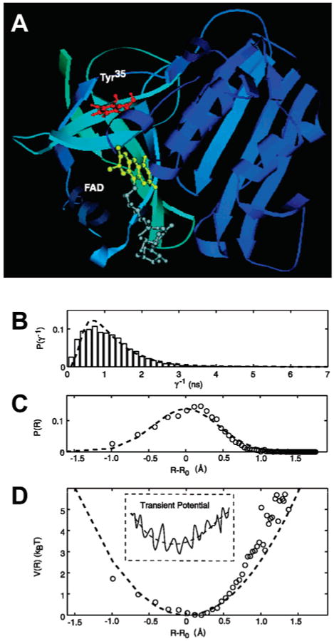
Enzyme conformational dynamics probes by ET. (A) Representative structure of the Fre/FAD complex from MD simulation. The fluorescent isoalloxazine moiety of FAD (yellow) sits in its binding pocket, in close proximity to the tyrosine residue (Tyr³⁵), which dominates the quenching of flavin fluorescence in Fre. (B) Distribution of fluorescence lifetimes obtained from a single-molecule time trace. (C) Distribution of the FAD–Tyr35 edge-to-edge distance derived from the distribution in part B using β = 1.4 Å⁻¹ in eq 14. (D) Potential of mean force calculated from part C. The dashed lines in all graphs correspond to fits to a harmonic potential of mean force around a center value R₀, and variance θ = 0.19 Ų. Inset: Sketch of a transient rugged potential for the protein conformational motion projected to the experimentally accessible coordinate R. Adapted with permission from Science (http://www.aaas.org), ref 31. Copyright 2003 American Association for the Advancement of Science.

5. Single-Molecule Protein Folding under Nonequilibrium Conditions

Single-molecule protein-folding experiments performed under equilibrium conditions are limited to the unfolding transition region where the various macrostates are substantially populated. The small population of unfolded protein molecules under native or nativelike conditions complicates the study of polypeptide chain collapse and increases the uncertainty in mean FRET efficiencies and the widths of FRET efficiency distributions and may obscure the detection of additional subpopulations, not present under more destabilizing conditions. Nonequilibrium conditions offer a convenient way to increase the population of unfolded species even under native or nativelike conditions.

For this purpose, Lipman et al.¹⁶⁸ combined a confocal single-molecule optical system with a microfluidic laminar mixing device etched on a silicon wafer. The design of the mixer was inspired by an earlier design by Kauffmann et al.,⁵⁸ who used it to study protein-folding kinetics at the ensemble level using infrared detection. By reducing the dimensions of the channels to several micrometers, these nanofabricated mixing devices enable efficient mixing solely by diffusion under conditions of laminar flow.^59,60 To demonstrate the performance of this device, Lipman et al. used Csp previously studied at the single-molecule level in solution.⁷⁰

By focusing a laser beam for sample excitation at various positions downstream of the mixing region, FRET efficiency histograms could be measured at various times after initiation of the refolding reaction by dilution of the denaturant by diffusion. E histograms of a typical refolding experiment are displayed in Figure 18A. Two different types of conformational transitions can be identified. First, there is a rapid shift in the mean E of the denatured subpopulation from ∼0.51 in the premixing region to ∼0.64 after the first 100 ms of initiation of the mixing process. This increase in E, which could not be time-resolved (the present technology does not allow observation of single molecules at these extremely short time scales because of the limited photon emission rate of the fluorophores used) is due to a rapid reconfigurational process of Csp to a more compact species in response to the new solvent conditions. This fast collapse phase is followed by a much slower process, which is characterized by a population redistribution of the collapsed denatured state and the folded native state. This process seems to be two-state, as the decrease in the denatured species is matched with a corresponding increase of the folded subpopulation. The rate of formation of the native state, obtained from fitting the change in the fraction of folded protein as a function of time to a single exponential function, was in excellent agreement with the single rate constant obtained from bulk stopped-flow experiments under identical solvent conditions, further reinforcing the two-state nature of the process. By changing the denaturant concentration in the refolding buffer, the authors could show that the mean E value of the denatured subpopulation increased nonlinearly from ∼0.5 at 3 M GdmCl or higher to 0.8 at 0.4 M GdmCl, a concentration outside the range accessible in their previous equilibrium–solution experiment (Figure 18C). Perhaps most surprising, no broadening in the width of the collapsed, denatured subpopulation was observed over the whole denaturant concentration tested and the peak position of the denatured subpopulation did not change during the folding reaction. Obviously, the reconfiguration rate of the unfolded state does not decrease under even strongly native conditions where the polypeptide adopts a substantially more compact conformation and a significant energy barrier remains.

Figure 18.

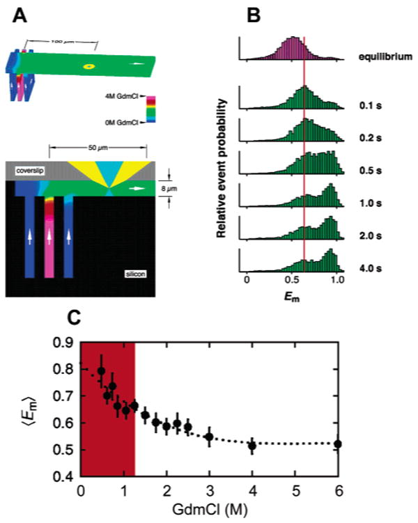
Probing single-molecule protein folding kinetics under nonequilibrium conditions. (A) Top: View of the mixing region of the microfluidic laminar mixing device, with the denaturant concentration indicated by a false color code. The laser beam (light blue) and collected fluorescence (yellow) are shown 100 μm from the center inlet. Bottom: Cross-section of the mixing region. (B) Histograms of measured FRET efficiency as a function of the mixing time. Within the first 100 ms of mixing, the expanded chain collapsed into a more compact coil structure, indicated by the slight increase in mean E. The collapsed denatured species reconfigure into the compact folded state on a time scale of a few seconds. Note that the mean E of the collapsed denatured subpopulation does not vary with time (red line) nor final denaturant concentration (data not shown). (C) Dependence of the mean E values of the collapsed coil state as a function of final denaturant concentration in the refolding buffer. The colored region highlights the denaturant range within which mean E values and distribution widths cannot be determined accurately using freely diffusing molecules under equilibrium conditions. Adapted with permission from Science (http://www.aaas.org), ref 168. Copyright 2003 American Association for the Advancement of Science.

6. Conclusion

The review presented here of recent single-molecule fluorescence studies of protein conformational fluctuations and folding/refolding at equilibrium or nonequilibrium is in no way exhaustive, as its purpose was to illustrate some general methods by a few characteristic recent examples. We nonetheless hope that it will entice the reader to follow some of the literature tracks started by, or linked to, each of the examples discussed here.

The lessons of these examples are twofold. First, single-molecule methods are for the most part reproducing results obtained at the ensemble level. This is important, as it means that artifacts due to the specific labeling, surface immobilization, type of spectroscopic techniques, etc. used in these approaches can be excluded if enough precautions are taken. We have mentioned a few cases where this is not true in order to emphasize the importance of ensemble/single-molecule comparison, and even comparison between different single-molecule experiments, to validate any new information extracted from these measurements. The extreme sensitivity of fluorophore emission to their environment or the small magnitude of forces needed to perturb biomolecules make it all too easy to confound photophysical effects or nonspecific interactions with the genuine signature of protein structural dynamics. As for any new methodology, a set of validation criteria will need to be established for comparison of results obtained by single-molecule methods with those obtained with other more established ones in their common domain of application. Photophysical effects (triplet state interconversion, blinking, isomerization, etc.) are usually well-diagnosed by excitation–intensity dependence studies, and nonspecific interactions can be excluded only when comparison with experiments on freely diffusing molecules can be provided or strong statistical unlikelihood of these effects can be demonstrated. A possible evolution of single-molecule methodology is to eventually replace some ensemble methods altogether, rendering validation mechanisms all the more crucial. Despite these concerns, our belief is that the current democratization of single-molecule methods (be it fluorescence-based or otherwise) will rapidly blend them into the standard toolkit of chemistry and biochemistry.

The second lesson is the power of single-molecule methods to uncover phenomena hidden at the ensemble level. This in itself will justify the efforts put into developing the validation criteria required for single-molecule methods to become mainstream tools. As illustrated by several examples along this review, studying single enzymes or fluctuating/folding proteins reveals a noticeable heterogeneity or dispersion of properties within a population that would be treated as a whole in ensemble studies. This heterogeneity can be in principle of two types: static or dynamic. As defined above, static heterogeneity of a property (or observable) corresponds to a situation where the measured property differs from one individual molecule to another but is well-defined in each case, whereas dynamic heterogeneity describes the more general case where each individual molecule exhibits a varying property. Dynamic heterogeneity might in fact be the general case, as static heterogeneity simply states the absence of dynamics on a time scale larger than the experimental time resolution (or smaller than the experiment duration).^210–212 The knowledge of the distribution of an observable (rather than just its average value, and possibly its variance, as obtained by ensemble measurements) is in any case sufficient to already gain insight into the behavior of the system, as exemplified by protein-folding studies at equilibrium. However, single-molecule studies of fluctuating proteins or enzymes have shown in addition that their dynamics can be highly nontrivial, often time exhibiting memory effects or non-Markovian character, as reported in several examples treated in this review. Theoretical models proposed to account for the observed dynamics are rather general (for instance, introducing multiple interconverting conformations or distribution of trapping times in an abstract energy landscape) and provide neither a clear picture of the exact conformations nor an indication of their potential biological function. Nevertheless, this new information provided solely by single-molecule approaches can be used to design novel assays aimed at elucidating the precise nature of these fluctuations.

The rapid pace of experimental and theoretical developments in single-molecule methods witnessed during the past few years is bound to continue, as many new directions remain to be explored. (i) Time-resolved fluorescence spectroscopy^31,105 provides information that can in principle be used to build 1D projections of protein energy landscapes (or more in case of multiple labeling schemes, see below). Although the theoretical literature is rich in models, methods will need to be developed to take full advantage of the experimental data and relate them to actual thermodynamic parameters.

(ii) The combination of different single-molecule techniques (e.g., electrophysiology and fluorescence,²¹³ force measurement,²¹⁴ or micromanipulation²¹⁵ and fluorescence) will permit correlation of conformational changes and catalytic step (or folding stage), allowing a complete description of many dynamic phenomena that remain currently inaccessible to molecular dynamic simulations.

(iii) Improvements in detector temporal³¹ and spatial²¹⁶ resolution should allow new dynamic regimes to be explored, as illustrated by lifetime fluctuation studies on immobilized molecules.³¹ Time- and space-resolved detectors, for instance, would allow one to follow single molecules in microfluidic devices¹⁶⁸ and monitor their trajectories in the specific phase space explored (distance between one or more pair of residues). For protein folding, this could give access to transient species in a way similar to that already observed at equilibrium on immobilized molecules^138,188 but now along the folding or unfolding pathway of individual molecules.

(iv) Labeling schemes involving multiple site-specific fluorophore attachment^{97,123,124,173} or new types of fluorophores having longer lifetimes and life spans (such as quantum dots^217–219) should allow difficult questions to be addressed more directly. In combination with the clear separation of subpopulations afforded by μs-ALEX, three-color (or four-color) FRET measurements would permit one to monitor three (or six) distances between intramolecular or intermolecular residues, extending the dimension of the projected phase space.

(v) In vivo single-molecule experiments^220–222 open the possibility to study enzyme activity or protein function in their native environment with the same sensitivity as in vitro single-molecule measurements, allowing one to check the biological relevance of these in vitro assays and uncover the influence of cellular crowding or unknown side effects.

Undoubtedly, single-molecule methods will continue to help deepen our understanding of biomolecular functions and contribute fundamental discoveries in biochemistry.

Biographies

Xavier Michalet received an Engineering Degree from Ecole Polytechnique (France), before getting acquainted with research in soft condensed matter under the supervision of David Bensimon at the Ecole Normale Supérieure. After his doctorate, he joined the group of Aaron Bensimon, with whom he developed genetic applications of DNA molecular combing. He joined Shimon Weiss's group at the Lawrence Berkeley National Laboratory, working on quantum dots applications to biology. He is now a project scientist at UCLA, working in the Weiss group on single-molecule studies of receptor diffusion, protein folding, mapping of transcription factor binding sites on whole genomes, and developing various techniques and detectors for single-molecule spectroscopy and microscopy.

Shimon Weiss is a Professor in the Department of Chemistry and Biochemistry and in the Department of Physiology at UCLA. He was previously a staff scientist at Lawrence Berkeley Labs, where, since 1991, he has been involved in nanoscale science and single-molecule spectroscopy. He pioneered research on single-molecule spectroscopy and its application to biology. His team was the first to detect FRET between a single donor and a single acceptor molecule, a technique that is now widely used to study the structure and conformational dynamics of macromolecules. He also pioneered the use of fluorescent semiconductor nanocrystals, or quantum dots, as biological probes, revolutionizing the use of fluorescence in modern biotechnology and cellular imaging. His group is currently involved in research on molecular imaging with quantum dots and single-molecule studies of transcription initiation, membrane receptor dynamic, and protein folding, among many others.

Marcus Jäger received the Diploma Degree in Biochemistry from the Freie Universität Berlin in 1994 and his Ph.D. from the University of Zurich in 2001 with Prof. Andreas Plückthun. From 2000 to 2002, he worked as a postdoctoral research associate with Prof. Jeffery W. Kelly at the Scripps Research Institute (La Jolla, California) and Prof. Martin Gruebele at the University of Illinois, Urbana—Champaign. Since 2002, he has been a member of the Single-Molecule Biophysics Group (Prof. Shimon Weiss) at UCLA, where he employs molecular biology, protein biochemistry, and single-molecule FRET to solve the protein folding problem.

References

- 1.Basché T, Moerner WE, Orrit M, Wild UP, editors. Single-Molecule Optical Detection, Imaging and Spectroscopy. VCH; Weinheim: 1997. [Google Scholar]
- 2.Nie S, Zare RN. Annu Rev Biophys Biomol Struct. 1997;26:567. doi: 10.1146/annurev.biophys.26.1.567. [DOI] [PubMed] [Google Scholar]
- 3.Xie XS, Trautman JK. Annu Rev Phys Chem. 1998;49:441. doi: 10.1146/annurev.physchem.49.1.441. [DOI] [PubMed] [Google Scholar]
- 4.Moerner WE, Orrit M. Science. 1999;283:1670. doi: 10.1126/science.283.5408.1670. [DOI] [PubMed] [Google Scholar]
- 5.Weiss S. Science. 1999;283:1676. doi: 10.1126/science.283.5408.1676. [DOI] [PubMed] [Google Scholar]
- 6.Weiss S. Nat Struct Biol. 2000;7:724. doi: 10.1038/78941. [DOI] [PubMed] [Google Scholar]
- 7.Michalet X, Weiss S. C R Phys. 2002;3:619. [Google Scholar]
- 8.Tinnefeld P, Sauer M. Angew Chem, Int Ed. 2005;44:2642. doi: 10.1002/anie.200300647. [DOI] [PubMed] [Google Scholar]
- 9.Kendrew JC. Nature. 1958;182:764. doi: 10.1038/182764a0. [DOI] [PubMed] [Google Scholar]
- 10.Perutz MF. Brookhaven Sym Biol. 1960;13:165. [PubMed] [Google Scholar]
- 11.Frauenfelder H, Wolynes PG. Science. 1985;229:337. doi: 10.1126/science.4012322. [DOI] [PubMed] [Google Scholar]
- 12.Ansari A, Berendzen J, Bowne SF, Frauenfelder H, Iben IE, Sauke TB, Shyamsunder E, Young RD. Proc Natl Acad Sci U S A. 1985;82:5000. doi: 10.1073/pnas.82.15.5000. [DOI] [PMC free article] [PubMed] [Google Scholar]
- 13.Frauenfelder H, Sligar SG, Wolynes PG. Science. 1991;254:1598. doi: 10.1126/science.1749933. [DOI] [PubMed] [Google Scholar]
- 14.Hvidt A, Nielsen SO. Adv Protein Chem. 1966;21:287. doi: 10.1016/s0065-3233(08)60129-1. [DOI] [PubMed] [Google Scholar]
- 15.Englander SW, Kallenbach NR. Q Rev Biophys. 1983;16:521. doi: 10.1017/s0033583500005217. [DOI] [PubMed] [Google Scholar]
- 16.Englander SW, Sosnick TR, Englander JJ, Mayne L. Curr Opin Struct Biol. 1996;6:18. doi: 10.1016/s0959-440x(96)80090-x. [DOI] [PMC free article] [PubMed] [Google Scholar]
- 17.Clarke J, Itzhaki LS. Curr Opin Struct Biol. 1998;8:112. doi: 10.1016/s0959-440x(98)80018-3. [DOI] [PubMed] [Google Scholar]
- 18.Shoemaker BA, Portman JJ, Wolynes PG. Proc Natl Acad Sci U S A. 2000;97:8868. doi: 10.1073/pnas.160259697. [DOI] [PMC free article] [PubMed] [Google Scholar]
- 19.Dunker AK, Brown CJ, Obradovic Z. Adv Protein Chem. 2002;62:25. doi: 10.1016/s0065-3233(02)62004-2. [DOI] [PubMed] [Google Scholar]
- 20.Dyson HJ, Wright PE. Chem Rev. 2004;104:3607. doi: 10.1021/cr030403s. [DOI] [PubMed] [Google Scholar]
- 21.Gutin AM, Abkevich VI, Shakhnovich EI. Biochemistry. 1995;34:3066. doi: 10.1021/bi00009a038. [DOI] [PubMed] [Google Scholar]
- 22.Eggers DK, Valentine JS. J Mol Biol. 2001;314:911. doi: 10.1006/jmbi.2001.5166. [DOI] [PubMed] [Google Scholar]
- 23.Ellis RJ. Curr Biol. 1997;7:R531. doi: 10.1016/s0960-9822(06)00273-9. [DOI] [PubMed] [Google Scholar]
- 24.Neri D, Billeter M, Wider G, Wuthrich K. Science. 1992;257:1559. doi: 10.1126/science.1523410. [DOI] [PubMed] [Google Scholar]
- 25.Logan TM, Theriault Y, Fesik SW. J Mol Biol. 1994;236:637. doi: 10.1006/jmbi.1994.1173. [DOI] [PubMed] [Google Scholar]
- 26.Shortle D, Ackerman MS. Science. 2001;293:487. doi: 10.1126/science.1060438. [DOI] [PubMed] [Google Scholar]
- 27.Shortle D. FASEB J. 1996;10:27. doi: 10.1096/fasebj.10.1.8566543. [DOI] [PubMed] [Google Scholar]
- 28.Anfinsen CB. Science. 1973;181:223. doi: 10.1126/science.181.4096.223. [DOI] [PubMed] [Google Scholar]
- 29.Privalov PL. Adv Protein Chem. 1982;35:1. [PubMed] [Google Scholar]
- 30.Garcia-Mira MM, Sadqi M, Fischer N, Sanchez-Ruiz JM, Munoz V. Science. 2002;298:2191. doi: 10.1126/science.1077809. [DOI] [PubMed] [Google Scholar]
- 31.Yang H, Luo G, Karnchanaphanurach P, Louie TM, Rech I, Cova S, Xun L, Xie XS. Science. 2003;302:262. doi: 10.1126/science.1086911. [DOI] [PubMed] [Google Scholar]
- 32.Tanford C. Adv Protein Chem. 1968;23:121. doi: 10.1016/s0065-3233(08)60401-5. [DOI] [PubMed] [Google Scholar]
- 33.Tanford C. Adv Protein Chem. 1970;24:1. [PubMed] [Google Scholar]
- 34.Kim PS, Baldwin RL. Annu Rev Biochem. 1982;51:459. doi: 10.1146/annurev.bi.51.070182.002331. [DOI] [PubMed] [Google Scholar]
- 35.Kim PS, Baldwin RL. Annu Rev Biochem. 1990;59:631. doi: 10.1146/annurev.bi.59.070190.003215. [DOI] [PubMed] [Google Scholar]
- 36.Jackson SE, Fersht AR. Biochemistry. 1991;30:10428. doi: 10.1021/bi00107a010. [DOI] [PubMed] [Google Scholar]
- 37.Alexander P, Fahnestock S, Lee T, Orban J, Bryan P. Biochemistry. 1992;31:3597. doi: 10.1021/bi00129a007. [DOI] [PubMed] [Google Scholar]
- 38.Jackson SE. Fold Des. 1998;3:R81. doi: 10.1016/S1359-0278(98)00033-9. [DOI] [PubMed] [Google Scholar]
- 39.Bryngelson JD, Onuchic JN, Socci ND, Wolynes PG. Proteins. 1995;21:167. doi: 10.1002/prot.340210302. [DOI] [PubMed] [Google Scholar]
- 40.Dill KA, Chan HS. Nat Struct Biol. 1997;4:10. doi: 10.1038/nsb0197-10. [DOI] [PubMed] [Google Scholar]
- 41.Onuchic JN, Luthey-Schulten Z, Wolynes PG. Annu Rev Phys Chem. 1997;48:545. doi: 10.1146/annurev.physchem.48.1.545. [DOI] [PubMed] [Google Scholar]
- 42.Itzhaki LS, Neira JL, Ruiz-Sanz J, de Prat Gay G, Fersht AR. J Mol Biol. 1995;254:289. doi: 10.1006/jmbi.1995.0617. [DOI] [PubMed] [Google Scholar]
- 43.Daggett V, Fersht AR. Trends Biochem Sci. 2003;28:18. doi: 10.1016/s0968-0004(02)00012-9. [DOI] [PubMed] [Google Scholar]
- 44.Klimov DK, Thirumalai D. J Mol Biol. 1998;282:471. doi: 10.1006/jmbi.1998.1997. [DOI] [PubMed] [Google Scholar]
- 45.Klimov DK, Thirumalai D. Proteins. 2001;43:465. doi: 10.1002/prot.1058. [DOI] [PubMed] [Google Scholar]
- 46.Shoemaker BA, Wang J, Wolynes PG. J Mol Biol. 1999;287:675. doi: 10.1006/jmbi.1999.2613. [DOI] [PubMed] [Google Scholar]
- 47.Bryngelson JD, Wolynes PG. Proc Natl Acad Sci U S A. 1987;84:7524. doi: 10.1073/pnas.84.21.7524. [DOI] [PMC free article] [PubMed] [Google Scholar]
- 48.Goto Y, Calciano LJ, Fink AL. Proc Natl Acad Sci U S A. 1990;87:573. doi: 10.1073/pnas.87.2.573. [DOI] [PMC free article] [PubMed] [Google Scholar]
- 49.Pande VS, Rokhsar DS. Proc Natl Acad Sci U S A. 1998;95:1490. doi: 10.1073/pnas.95.4.1490. [DOI] [PMC free article] [PubMed] [Google Scholar]
- 50.Alonso DO, Dill KA, Stigter D. Biopolymers. 1991;31:1631. doi: 10.1002/bip.360311317. [DOI] [PubMed] [Google Scholar]
- 51.Roder H, Colon W. Curr Opin Struct Biol. 1997;7:15. doi: 10.1016/s0959-440x(97)80004-8. [DOI] [PubMed] [Google Scholar]
- 52.Capaldi AP, Shastry MC, Kleanthous C, Roder H, Radford SE. Nat Struct Biol. 2001;8:68. doi: 10.1038/83074. [DOI] [PubMed] [Google Scholar]
- 53.Heidary DK, Gross LA, Roy M, Jennings PA. Nat Struct Biol. 1997;4:725. doi: 10.1038/nsb0997-725. [DOI] [PubMed] [Google Scholar]
- 54.Teilum K, Maki K, Kragelund BB, Poulsen FM, Roder H. Proc Natl Acad Sci U S A. 2002;99:9807. doi: 10.1073/pnas.152321499. [DOI] [PMC free article] [PubMed] [Google Scholar]
- 55.Baldwin RL. Fold Des. 1996;1:R1. doi: 10.1016/S1359-0278(96)00003-X. [DOI] [PubMed] [Google Scholar]
- 56.Gruebele M. Curr Opin Struct Biol. 2002;12:161. doi: 10.1016/s0959-440x(02)00304-4. [DOI] [PubMed] [Google Scholar]
- 57.Shastry MC, Luck SD, Roder H. Biophys J. 1998;74:2714. doi: 10.1016/S0006-3495(98)77977-9. [DOI] [PMC free article] [PubMed] [Google Scholar]
- 58.Kauffmann E, Darnton NC, Austin RH, Batt C, Gerwert K. Proc Natl Acad Sci U S A. 2001;98:6646. doi: 10.1073/pnas.101122898. [DOI] [PMC free article] [PubMed] [Google Scholar]
- 59.Pabit SA, Hagen SJ. Biophys J. 2002;83:2872. doi: 10.1016/S0006-3495(02)75296-X. [DOI] [PMC free article] [PubMed] [Google Scholar]
- 60.Hertzog DE, Michalet X, Jager M, Kong X, Santiago JG, Weiss S, Bakajin O. Anal Chem. 2004;76:7169. doi: 10.1021/ac048661s. [DOI] [PMC free article] [PubMed] [Google Scholar]
- 61.Ballew RM, Sabelko J, Gruebele M. Proc Natl Acad Sci U S A. 1996;93:5759. doi: 10.1073/pnas.93.12.5759. [DOI] [PMC free article] [PubMed] [Google Scholar]
- 62.Munoz V, Thompson PA, Hofrichter J, Eaton WA. Nature. 1997;390:196. doi: 10.1038/36626. [DOI] [PubMed] [Google Scholar]
- 63.Jacob M, Holtermann G, Perl D, Reinstein J, Schindler T, Geeves MA, Schmid FX. Biochemistry. 1999;38:2882. doi: 10.1021/bi982487i. [DOI] [PubMed] [Google Scholar]
- 64.Jones CM, Henry ER, Hu Y, Chan CK, Luck SD, Bhuyan A, Roder H, Hofrichter J, Eaton WA. Proc Natl Acad Sci U S A. 1993;90:11860. doi: 10.1073/pnas.90.24.11860. [DOI] [PMC free article] [PubMed] [Google Scholar]
- 65.Hagen SJ, Hofrichter J, Szabo A, Eaton WA. Proc Natl Acad Sci U S A. 1996;93:11615. doi: 10.1073/pnas.93.21.11615. [DOI] [PMC free article] [PubMed] [Google Scholar]
- 66.Sabelko J, Ervin J, Gruebele M. Proc Natl Acad Sci U S A. 1999;96:6031. doi: 10.1073/pnas.96.11.6031. [DOI] [PMC free article] [PubMed] [Google Scholar]
- 67.Huang CY, Getahun Z, Zhu Y, Klemke JW, DeGrado WF, Gai F. Proc Natl Acad Sci U S A. 2002;99:2788. doi: 10.1073/pnas.052700099. [DOI] [PMC free article] [PubMed] [Google Scholar]
- 68.Leeson DT, Gai F, Rodriguez HM, Gregoret LM, Dyer RB. Proc Natl Acad Sci U S A. 2000;97:2527. doi: 10.1073/pnas.040580397. [DOI] [PMC free article] [PubMed] [Google Scholar]
- 69.Yang WY, Gruebele M. Biophys J. 2004;87:596. doi: 10.1529/biophysj.103.039040. [DOI] [PMC free article] [PubMed] [Google Scholar]
- 70.Schuler B, Lipman EA, Eaton WA. Nature. 2002;419:743. doi: 10.1038/nature01060. [DOI] [PubMed] [Google Scholar]
- 71.Haas E, Katchalski-Katzir E, Steinberg IZ. Biochemistry. 1978;17:5064. doi: 10.1021/bi00616a032. [DOI] [PubMed] [Google Scholar]
- 72.Lapidus LJ, Eaton WA, Hofrichter J. Phys Rev Lett. 2001;87:258101. doi: 10.1103/PhysRevLett.87.258101. [DOI] [PubMed] [Google Scholar]
- 73.Buscaglia M, Schuler B, Lapidus LJ, Eaton WA, Hofrichter J. J Mol Biol. 2003;332:9. doi: 10.1016/s0022-2836(03)00891-x. [DOI] [PubMed] [Google Scholar]
- 74.Bieri O, Wirz J, Hellrung B, Schutkowski M, Drewello M, Kiefhaber T. Proc Natl Acad Sci U S A. 1999;96:9597. doi: 10.1073/pnas.96.17.9597. [DOI] [PMC free article] [PubMed] [Google Scholar]
- 75.Krieger F, Fierz B, Bieri O, Drewello M, Kiefhaber T. J Mol Biol. 2003;332:265. doi: 10.1016/s0022-2836(03)00892-1. [DOI] [PubMed] [Google Scholar]
- 76.Kubelka J, Hofrichter J, Eaton WA. Curr Opin Struct Biol. 2004;14:76. doi: 10.1016/j.sbi.2004.01.013. [DOI] [PubMed] [Google Scholar]
- 77.Hass E. ChemPhysChem. 2005;6:858. [Google Scholar]
- 78.Lakowicz JR. Principles of Fluorescence Spectroscopy. 2nd. Plenum; New York: 1999. [Google Scholar]
- 79.Tinnefeld P, Buschmann V, Weston KD, Sauer M. J Phys Chem A. 2003;107:323. [Google Scholar]
- 80.Zander C, Enderlein J, Keller RA. Single Molecule Detection in Solution: Methods and Applications. Wiley-VCH; New York: 2002. [Google Scholar]
- 81.Barkai E, Jung Y, Silbey R. Annu Rev Phys Chem. 2004;55:457. doi: 10.1146/annurev.physchem.55.111803.143246. [DOI] [PubMed] [Google Scholar]
- 82.Koshioka M, Sasaki K, Masuhara H. Appl Spectrosc. 1995;49:224. [Google Scholar]
- 83.Ha T, Laurence TA, Chemla DS, Weiss S. J Phys Chem B. 1999;103:6839. [Google Scholar]
- 84.Forkey JN, Quinlan ME, Goldman YE. Prog Biophys Mol Biol. 2000;74:1. doi: 10.1016/s0079-6107(00)00015-8. [DOI] [PubMed] [Google Scholar]
- 85.Kinosita K, Adachi K, Itoh H. Annu Rev Biophys Biomol Struct. 2004;33:245. doi: 10.1146/annurev.biophys.33.110502.132716. [DOI] [PubMed] [Google Scholar]
- 86.Rosenberg SA, Quinlan ME, Forkey JN, Goldman YE. Acc Chem Res. 2005;38:583. doi: 10.1021/ar040137k. [DOI] [PubMed] [Google Scholar]
- 87.Van der Meer BW, Coker GI, Chen SYS. Resonance Energy Transfer: Theory and Data. Wiley-VCH; New York: 1991. [Google Scholar]
- 88.Förster T. Ann Phys. 1948;6:55. [Google Scholar]
- 89.Stryer L, Haugland RP. Proc Natl Acad Sci U S A. 1967;58:719. doi: 10.1073/pnas.58.2.719. [DOI] [PMC free article] [PubMed] [Google Scholar]
- 90.Ha T, Enderle T, Ogletree DF, Chemla DS, Selvin PR, Weiss S. Proc Natl Acad Sci U S A. 1996;93:6264. doi: 10.1073/pnas.93.13.6264. [DOI] [PMC free article] [PubMed] [Google Scholar]
- 91.Deniz AA, Dahan M, Grunwell JR, Ha T, Faulhaber AE, Chemla DS, Weiss S, Schultz PG. Proc Natl Acad Sci U S A. 1999;96:3670. doi: 10.1073/pnas.96.7.3670. [DOI] [PMC free article] [PubMed] [Google Scholar]
- 92.Marcus RA, Sutin N. Biochim Biophys Acta. 1985;811:265. [Google Scholar]
- 93.Moser CC, Keske JM, Warncke K, Farid RS, Dutton PL. Nature. 1992;355:796. doi: 10.1038/355796a0. [DOI] [PubMed] [Google Scholar]
- 94.Neuweiler H, Schulz A, Böhmer M, Enderlein J, Sauer M. J Am Chem Soc. 2003;125:5324. doi: 10.1021/ja034040p. [DOI] [PubMed] [Google Scholar]
- 95.Wang H, Luo G, Karnchanaphanurach P, Louie TM, Cova S, Xun L, Xie XS. Science. 2003;302:262. doi: 10.1126/science.1086911. [DOI] [PubMed] [Google Scholar]
- 96.Eggeling C, Volkmer A, Seidel CAM. ChemPhysChem. 2005;6:791. doi: 10.1002/cphc.200400509. [DOI] [PubMed] [Google Scholar]
- 97.Kapanidis AN, Weiss S. J Chem Phys. 2002;117:10953. [Google Scholar]
- 98.Pawley JB, editor. Handbook of Biological Confocal Microscopy. 2nd. Plenum Press; New York: 1995. [Google Scholar]
- 99.Michalet X, Kapanidis AN, Laurence T, Pinaud F, Doose S, Pflughoefft M, Weiss S. Ann Rev Biophys Biomol Struct. 2003;32:161. doi: 10.1146/annurev.biophys.32.110601.142525. [DOI] [PubMed] [Google Scholar]
- 100.Zhuang X, Rief M. Curr Opin Struct Biol. 2003;13:88. doi: 10.1016/s0959-440x(03)00011-3. [DOI] [PubMed] [Google Scholar]
- 101.Haran G. J Phys: Condens Mater. 2003;15:R1291. [Google Scholar]
- 102.Moerner WE, Fromm DP. Rev Sci Instrum. 2003;74:3597. [Google Scholar]
- 103.Rothwell PJ, Berger S, Kensch O, Felekyan S, Antonik M, Wo BM, Restle T, Goody RS, Seidel CAM. Proc Natl Acad Sci U S A. 2003;100:1655. doi: 10.1073/pnas.0434003100. [DOI] [PMC free article] [PubMed] [Google Scholar]
- 104.Margittai M, Widengren J, Schweinberger E, Schröder GF, Felekyan S, Haustein E, König M, Fasshauer D, Grubmüller H, Jahn R, Seidel CAM. Proc Natl Acad Sci U S A. 2003;100:15516. doi: 10.1073/pnas.2331232100. [DOI] [PMC free article] [PubMed] [Google Scholar]
- 105.Laurence TA, Kong X, Jäger M, Weiss S. Proc Natl Acad Sci U S A. 2005;102:17348. doi: 10.1073/pnas.0508584102. [DOI] [PMC free article] [PubMed] [Google Scholar]
- 106.Kinosita K, Itoh H, Ishiwata Si, Hirano Ki, Nishizaka T, Hayakawa T. J Cell Biol. 1991;115:67. doi: 10.1083/jcb.115.1.67. [DOI] [PMC free article] [PubMed] [Google Scholar]
- 107.Cognet L, Harms GS, Blab GA, Lommerse PHM, Schmidt T. Appl Phys Lett. 2000;77:4052. [Google Scholar]
- 108.Blab GA, Oellerich S, Schumm R, Schmidt T. Opt Lett. 2004;29:727. doi: 10.1364/ol.29.000727. [DOI] [PubMed] [Google Scholar]
- 109.Michalet X, Siegmund OHW, Vallerga JV, Jelinsky P, Millaud JE, Weiss S. J Mod Optics. in press. [Google Scholar]
- 110.Deniz AA, Laurence TA, Beligere GS, Dahan M, Martin AB, Chemla DS, Dawson PE, Schultz PG, Weiss S. Proc Natl Acad Sci U S A. 2000;97:5179. doi: 10.1073/pnas.090104997. [DOI] [PMC free article] [PubMed] [Google Scholar]
- 111.Kapanidis AN, Lee NK, Laurence TA, Doose S, Margeat E, Weiss S. Proc Natl Acad Sci U S A. 2004;101:8936. doi: 10.1073/pnas.0401690101. [DOI] [PMC free article] [PubMed] [Google Scholar]
- 112.Kapanidis AN, Laurence TA, Lee NK, Margeat E, Kong X, Weiss S. Acc Chem Res. 2005;38:523. doi: 10.1021/ar0401348. [DOI] [PubMed] [Google Scholar]
- 113.Li H, Ren X, Ying L, Balasubramanian S, Klenerman D. Proc Natl Acad Sci U S A. 2004;101:14425. doi: 10.1073/pnas.0404295101. [DOI] [PMC free article] [PubMed] [Google Scholar]
- 114.Müller BK, Zaychikov E, Bräuchle C, Lamb DC. Biophys J. 2005;89:3508. doi: 10.1529/biophysj.105.064766. [DOI] [PMC free article] [PubMed] [Google Scholar]
- 115.Dahan M, Deniz AA, Ha T, Chemla DS, Schultz PG, Weiss S. Chem Phys. 1999;247:85. [Google Scholar]
- 116.Böhmer M, Pampaloni F, Wahl M, Rahn HJ, Erdmann R, Enderlein J. Rev Sci Instrum. 2001;72:4145. [Google Scholar]
- 117.Felekyan S, Kuhnemuth R, Kudryavtsev V, Sandhagen C, Becker W, Seidel CAM. Rev Sci Instrum. 2005;76:083104. [Google Scholar]
- 118.Ha T, Ting AY, Liang J, Caldwell WB, Deniz AA, Chemla DS, Schultz PG, Weiss S. Proc Natl Acad Sci U S A. 1999;96:893. doi: 10.1073/pnas.96.3.893. [DOI] [PMC free article] [PubMed] [Google Scholar]
- 119.Lee NK, Kapanidis AN, Wang Y, Michalet X, Mukhopadhyay J, Ebright RH, Weiss S. Biophys J. 2005;88:2939. doi: 10.1529/biophysj.104.054114. [DOI] [PMC free article] [PubMed] [Google Scholar]
- 120.Ramirez-Carrozzi V, Kerppola T. Methods. 2001;25:31. doi: 10.1006/meth.2001.1213. [DOI] [PubMed] [Google Scholar]
- 121.Haustein E, Jahnz M, Schwille P. ChemPhysChem. 2003;4:745. doi: 10.1002/cphc.200200634. [DOI] [PubMed] [Google Scholar]
- 122.Watrob HM, Pan CP, Barkley MD. J Am Chem Soc. 2003;125:7336. doi: 10.1021/ja034564p. [DOI] [PubMed] [Google Scholar]
- 123.Hohng S, Joo C, Ha T. Biophys J. 2004;87:1328. doi: 10.1529/biophysj.104.043935. [DOI] [PMC free article] [PubMed] [Google Scholar]
- 124.Clamme JP, Deniz AA. ChemPhysChem. 2005;6:74. doi: 10.1002/cphc.200400261. [DOI] [PubMed] [Google Scholar]
- 125.Heilemann M, Tinnefeld P, Mosteiro GS, Parajo MG, Van Hulst NF, Sauer M. J Am Chem Soc. 2004;126:6514. doi: 10.1021/ja049351u. [DOI] [PubMed] [Google Scholar]
- 126.Lu HP, Xun L, Xie XS. Science. 1998;282:1877. doi: 10.1126/science.282.5395.1877. [DOI] [PubMed] [Google Scholar]
- 127.Jia Y, Talaga DS, Lau WL, Lu HSM, DeGrado WF, Hochstrasser RM. Chem Phys. 1999;247:69. [Google Scholar]
- 128.Elson EL, Magde D. Biopolymers. 1974;13:1. doi: 10.1002/bip.1974.360130103. [DOI] [PubMed] [Google Scholar]
- 129.Rigler R, Elson ES, editors. Fluorescence Correlation Spectroscopy. Theory and Applications. Springer; New York: 2001. [Google Scholar]
- 130.Krichevsky O, Bonnet G. Rep Prog Phys. 2002;65:251. [Google Scholar]
- 131.Chen Y, Müller JD, So PT, Gratton E. Biophys J. 1999;77:553. doi: 10.1016/S0006-3495(99)76912-2. [DOI] [PMC free article] [PubMed] [Google Scholar]
- 132.Palo K, Metz U, Jager S, Kask P, Gall K. Biophys J. 2000;76:2858. doi: 10.1016/S0006-3495(00)76523-4. [DOI] [PMC free article] [PubMed] [Google Scholar]
- 133.Laurence TA, Kapanidis AN, Kong XX, Chemla DS, Weiss S. J Phys Chem B. 2004;108:3051. [Google Scholar]
- 134.Berglund AJ, Doherty AC, Mabuchi H. Phys Rev Lett. 2002;89:068101. doi: 10.1103/PhysRevLett.89.068101. [DOI] [PubMed] [Google Scholar]
- 135.Ariunbold GO, Agarwal GS, Wang Z, Scully MO, Walther H. J Phys Chem A. 2004;108:2402. [Google Scholar]
- 136.Gopich IV, Szabo A. J Phys Chem B. 2003;107:5058. [Google Scholar]
- 137.Gopich IV, Szabo A. J Chem Phys. 2005;122:014707. doi: 10.1063/1.1812746. [DOI] [PubMed] [Google Scholar]
- 138.Rhoades E, Gussakovsky E, Haran G. Proc Natl Acad Sci U S A. 2003;100:3197. doi: 10.1073/pnas.2628068100. [DOI] [PMC free article] [PubMed] [Google Scholar]
- 139.Talaga DS, Lau WL, Roder H, Tang J, Jia Y, DeGrado WF, Hochstrasser RM. Proc Natl Acad Sci U S A. 2000;97:13021. doi: 10.1073/pnas.97.24.13021. [DOI] [PMC free article] [PubMed] [Google Scholar]
- 140.Haran G. Chem Phys. 2004;307:137. [Google Scholar]
- 141.Chung SH, Kennedy RA. J Neurosci Methods. 1991;40:71. doi: 10.1016/0165-0270(91)90118-j. [DOI] [PubMed] [Google Scholar]
- 142.Deniz AA, Laurence TA, Dahan M, Chemla DS, Schultz PG, Weiss S. Annu Rev Phys Chem. 2001;52:233–253. doi: 10.1146/annurev.physchem.52.1.233. [DOI] [PubMed] [Google Scholar]
- 143.Schröder GF, Grubmüller H. J Chem Phys. 2003;119:9920. [Google Scholar]
- 144.Watkins LP, Yang H. Biophys J. 2004;86:4015. doi: 10.1529/biophysj.103.037739. [DOI] [PMC free article] [PubMed] [Google Scholar]
- 145.Watkins LP, Yang H. J Phys Chem B. 2005;109:617. doi: 10.1021/jp0467548. [DOI] [PubMed] [Google Scholar]
- 146.Andrec M, Levy RM, Talaga DS. J Phys Chem A. 2003;107:7454. doi: 10.1021/jp035514+. [DOI] [PMC free article] [PubMed] [Google Scholar]
- 147.Kazmirski SL, Wong KB, Freund SM, Tan YJ, Fersht AR, Daggett V. Proc Natl Acad Sci U S A. 2001;98:4349. doi: 10.1073/pnas.071054398. [DOI] [PMC free article] [PubMed] [Google Scholar]
- 148.Li A, Daggett V. Proc Natl Acad Sci U S A. 1994;91:10430. doi: 10.1073/pnas.91.22.10430. [DOI] [PMC free article] [PubMed] [Google Scholar]
- 149.Li A, Daggett V. J Mol Biol. 1996;257:412. doi: 10.1006/jmbi.1996.0172. [DOI] [PubMed] [Google Scholar]
- 150.Daggett V, Li A, Itzhaki LS, Otzen DE, Fersht AR. J Mol Biol. 1996;257:430. doi: 10.1006/jmbi.1996.0173. [DOI] [PubMed] [Google Scholar]
- 151.Otzen DE, Itzhaki LS, El Masry NF, Jackson SE, Fersht AR. Proc Natl Acad Sci U S A. 1994;91:10422. doi: 10.1073/pnas.91.22.10422. [DOI] [PMC free article] [PubMed] [Google Scholar]
- 152.Lazaridis T, Karplus M. Science. 1997;278:1928. doi: 10.1126/science.278.5345.1928. [DOI] [PubMed] [Google Scholar]
- 153.Ladurner AG, Itzhaki LS, Daggett V, Fersht AR. Proc Natl Acad Sci U S A. 1998;95:8473. doi: 10.1073/pnas.95.15.8473. [DOI] [PMC free article] [PubMed] [Google Scholar]
- 154.de Prat Gay G, Ruiz-Sanz J, Davis B, Fersht AR. Proc Natl Acad Sci U S A. 1994;91:10943. doi: 10.1073/pnas.91.23.10943. [DOI] [PMC free article] [PubMed] [Google Scholar]
- 155.de Prat Gay G, Ruiz-Sanz J, Neira JL, Itzhaki LS, Fersht AR. Proc Natl Acad Sci U S A. 1995;92:3683. doi: 10.1073/pnas.92.9.3683. [DOI] [PMC free article] [PubMed] [Google Scholar]
- 156.Neira JL, Itzhaki LS, Ladurner AG, Davis B, de Prat Gay G, Fersht AR. J Mol Biol. 1997;268:185. doi: 10.1006/jmbi.1997.0932. [DOI] [PubMed] [Google Scholar]
- 157.Muir TW, Sondhi D, Cole PA. Proc Natl Acad Sci U S A. 1998;95:6705. doi: 10.1073/pnas.95.12.6705. [DOI] [PMC free article] [PubMed] [Google Scholar]
- 158.Dawson PE, Muir TW, Clark-Lewis I, Kent SB. Science. 1994;266:776. doi: 10.1126/science.7973629. [DOI] [PubMed] [Google Scholar]
- 159.Ladurner AG, Itzhaki LS, de Prat Gay G, Fersht AR. J Mol Biol. 1997;273:317. doi: 10.1006/jmbi.1997.1303. [DOI] [PubMed] [Google Scholar]
- 160.Santoro MM, Bolen DW. Biochemistry. 1988;27:8063. doi: 10.1021/bi00421a014. [DOI] [PubMed] [Google Scholar]
- 161.Perl D, Jacob M, Bano M, Stupak M, Antalik M, Schmid FX. Biophys Chem. 2002;96:173. doi: 10.1016/s0301-4622(02)00024-8. [DOI] [PubMed] [Google Scholar]
- 162.Schindler T, Herrler M, Marahiel MA, Schmid FX. Nat Struct Biol. 1995;2:663. doi: 10.1038/nsb0895-663. [DOI] [PubMed] [Google Scholar]
- 163.Ratner V, Kahana E, Eichler M, Haas E. Bioconjugate Chem. 2002;13:1163. doi: 10.1021/bc025537b. [DOI] [PubMed] [Google Scholar]
- 164.Plaxco KW, Millett IS, Segel DJ, Doniach S, Baker D. Nat Struct Biol. 1999;6:554. doi: 10.1038/9329. [DOI] [PubMed] [Google Scholar]
- 165.Jacob J, Krantz B, Dothager RS, Thiyagarajan P, Sosnick TR. J Mol Biol. 2004;338:369. doi: 10.1016/j.jmb.2004.02.065. [DOI] [PubMed] [Google Scholar]
- 166.Jacob M, Schmid FX. Biochemistry. 1999;38:13773. doi: 10.1021/bi991503o. [DOI] [PubMed] [Google Scholar]
- 167.Schuler B, Lipman EA, Steinbach PJ, Kumke M, Eaton WA. Proc Natl Acad Sci U S A. 2005;102:2754. doi: 10.1073/pnas.0408164102. [DOI] [PMC free article] [PubMed] [Google Scholar]
- 168.Lipman EA, Schuler B, Bakajin O, Eaton WA. Science. 2003;301:1233. doi: 10.1126/science.1085399. [DOI] [PubMed] [Google Scholar]
- 169.Eaton WA. Proc Natl Acad Sci U S A. 1999;96:5897. doi: 10.1073/pnas.96.11.5897. [DOI] [PMC free article] [PubMed] [Google Scholar]
- 170.Amirgoulova EV, Groll J, Heyes CD, Ameringer T, Rocker C, Moller M, Nienhaus GU. ChemPhysChem. 2004;5:552. doi: 10.1002/cphc.200400024. [DOI] [PubMed] [Google Scholar]
- 171.Groll J, Amirgoulova EV, Ameringer T, Heyes CD, Rocker C, Nienhaus GU, Moller M. J Am Chem Soc. 2004;126:4234. doi: 10.1021/ja0318028. [DOI] [PubMed] [Google Scholar]
- 172.Zhuang X, Kim H, Pereira MJ, Babcock HP, Walter NG, Chu S. Science. 2002;296:1473. doi: 10.1126/science.1069013. [DOI] [PubMed] [Google Scholar]
- 173.Jäger M, Michalet X, Weiss S. Protein Sci. 2005;14:2059. doi: 10.1110/ps.051384705. [DOI] [PMC free article] [PubMed] [Google Scholar]
- 174.Ladurner AG, Fersht AR. Nat Struct Biol. 1999;6:28. doi: 10.1038/4899. [DOI] [PubMed] [Google Scholar]
- 175.Jacob M, Schindler T, Balbach J, Schmid FX. Proc Natl Acad Sci U S A. 1997;94:5622. doi: 10.1073/pnas.94.11.5622. [DOI] [PMC free article] [PubMed] [Google Scholar]
- 176.Chirico G, Cannone F, Beretta S, Diaspro A, Campanini B, Bettati S, Ruotolo R, Mozzarelli A. Protein Sci. 2002;11:1152. doi: 10.1110/ps.4490102. [DOI] [PMC free article] [PubMed] [Google Scholar]
- 177.Dickson RM, Norris DJ, Tzeng YL, Moerner WE. Science. 1996;274:966. doi: 10.1126/science.274.5289.966. [DOI] [PubMed] [Google Scholar]
- 178.Yang S, Cao J. J Chem Phys. 2004;121:572. doi: 10.1063/1.1756578. [DOI] [PubMed] [Google Scholar]
- 179.Okumus B, Wilson TJ, Lilley DM, Ha T. Biophys J. 2004;87:2798. doi: 10.1529/biophysj.104.045971. [DOI] [PMC free article] [PubMed] [Google Scholar]
- 180.Ha T, Ting AY, Deniz AA, Chemla DS, Schultz PG, Weiss S. Chem Phys. 1999;247:107. doi: 10.1073/pnas.96.3.893. [DOI] [PMC free article] [PubMed] [Google Scholar]
- 181.Chen Y, Hu D, Vorpagel ER, Lu HP. J Phys Chem B. 2003;107:7947. [Google Scholar]
- 182.Lu HP. Curr Pharm Biotechnol. 2004;5:261. doi: 10.2174/1389201043376887. [DOI] [PubMed] [Google Scholar]
- 183.Hu D, Lu HP. J Phys Chem B. 2003;107:618. [Google Scholar]
- 184.Brasselet S, Peterman EJG, Miyawaki A, Moerner WE. J Phys Chem B. 2000;104:3676. [Google Scholar]
- 185.Slaughter BD, Allen MW, Unruh JR, Bieber Urbauer RJ, Johnson CK. J Phys Chem B. 2004;108:10388. [Google Scholar]
- 186.Tang J, Mei E, Green C, Kaplan J, DeGrado WF, Smith AB, Hochstrasser RM. J Phys Chem B. 2004;108:15910. [Google Scholar]
- 187.Miyawaki A, Llopis J, Heim R, McCaffery JM, Adams JA, Ikurak M, Tsien RY. Nature. 1997;388:882. doi: 10.1038/42264. [DOI] [PubMed] [Google Scholar]
- 188.Rhoades E, Cohen M, Schuler B, Haran G. J Am Chem Soc. 2004;126:14686. doi: 10.1021/ja046209k. [DOI] [PubMed] [Google Scholar]
- 189.Bonnet G, Krichevsky O, Libchaber A. Proc Natl Acad Sci U S A. 1998;95:8602. doi: 10.1073/pnas.95.15.8602. [DOI] [PMC free article] [PubMed] [Google Scholar]
- 190.Zhuang X, Ha T, Kim HD, Centner T, Labeit S, Chu S. Proc Natl Acad Sci U S A. 2000;97:14241. doi: 10.1073/pnas.97.26.14241. [DOI] [PMC free article] [PubMed] [Google Scholar]
- 191.Grama L, Somogyi B, Kellermayer MSZ. Proc Natl Acad Sci U S A. 2001;98:14362. doi: 10.1073/pnas.191494098. [DOI] [PMC free article] [PubMed] [Google Scholar]
- 192.Kästner CN, Prummer M, Sick B, Renn A, Wild UP, Dimroth P. Biophys J. 2003;84:1651. doi: 10.1016/S0006-3495(03)74974-1. [DOI] [PMC free article] [PubMed] [Google Scholar]
- 193.Rief M, Gautel M, Oesterhelt F, Fernandez JM, Gaub HE. Science. 1997;276:1109. doi: 10.1126/science.276.5315.1109. [DOI] [PubMed] [Google Scholar]
- 194.Chattopadhyay K, Elson EL, Frieden C. Proc Natl Acad Sci U S A. 2005;102:2385. doi: 10.1073/pnas.0500127102. [DOI] [PMC free article] [PubMed] [Google Scholar]
- 195.Schenter GK, Lu HP, Xie XS. J Phys Chem A. 1999;103:10477. [Google Scholar]
- 196.Xue Q, Yeung ES. Nature. 1995;373:681. doi: 10.1038/373681a0. [DOI] [PubMed] [Google Scholar]
- 197.Craig DB, Arriaga EA, Wong JCY, Lu H, Dovichi NJ. J Am Chem Soc. 1996;118:5245. [Google Scholar]
- 198.Edman L, Földes-Papp Z, Wennmalm S, Rigler R. Chem Phys. 1999;247:11. [Google Scholar]
- 199.Edman L, Rigler R. Proc Natl Acad Sci U S A. 2000;97:8266. doi: 10.1073/pnas.130589397. [DOI] [PMC free article] [PubMed] [Google Scholar]
- 200.Velonia K, Flomenbom O, Loos D, Masuo S, Cotlet M, Engelborghs Y, Hofkens J, Rowan AE, Klafter J, Nolte RJM, de Schryver FC. Angew Chem, Int Ed. 2005;44:560. doi: 10.1002/anie.200460625. [DOI] [PubMed] [Google Scholar]
- 201.Flomenbom O, Velonia K, Loos D, Masuo S, Cotlet M, Engelborghs Y, Hofkens J, Rowan AE, Nolte RJM, Van der Auweraer M, de Schryver FC, Klafter J. Proc Natl Acad Sci U S A. 2005;102:2368. doi: 10.1073/pnas.0409039102. [DOI] [PMC free article] [PubMed] [Google Scholar]
- 202.Tan X, Hu D, Squier TC, Lu HP. Appl Phys Lett. 2004;85:2420. [Google Scholar]
- 203.Holman MW, Adams DM. ChemPhysChem. 2004;5:1831. doi: 10.1002/cphc.200400123. [DOI] [PubMed] [Google Scholar]
- 204.Edman L, Mets Ü, Rigler R. Proc Natl Acad Sci U S A. 1996;93:6710. doi: 10.1073/pnas.93.13.6710. [DOI] [PMC free article] [PubMed] [Google Scholar]
- 205.Lu HP, Xie XS. J Phys Chem B. 1997;101:2753. [Google Scholar]
- 206.Piestert O, Barsch H, Buschmann V, Heinlein T, Knemeyer JP, Weston KD, Sauer M. Nano Lett. 2003;3:979. [Google Scholar]
- 207.Yang H, Xie XS. J Chem Phys. 2002;117:10965. [Google Scholar]
- 208.Yang H, Xie XS. Chem Phys. 2002;284:423. [Google Scholar]
- 209.Kou SC, Xie XS. Phys Rev Lett. 2004;93:180603. doi: 10.1103/PhysRevLett.93.180603. [DOI] [PubMed] [Google Scholar]
- 210.Zwanzig R. Acc Chem Res. 1990;23:148. [Google Scholar]
- 211.Xie XS. Single Mol. 2001;2:229. [Google Scholar]
- 212.Xie XS. J Chem Phys. 2002;117:11024. [Google Scholar]
- 213.Sonnleitner A, Mannuzzu LM, Terakawa S, Isacoff EY. Proc Natl Acad Sci U S A. 2002;99:12759. doi: 10.1073/pnas.192261499. [DOI] [PMC free article] [PubMed] [Google Scholar]
- 214.Sarkar A, Robertson RR, Fernandez JM. Proc Natl Acad Sci U S A. 2004;101:12882. doi: 10.1073/pnas.0403534101. [DOI] [PMC free article] [PubMed] [Google Scholar]
- 215.Rondelez Y, Tresset G, Nakashima T, Kato-Yamada Y, Fujita H, Takeuchi S, Noji H. Nature. 2005;433:773. doi: 10.1038/nature03277. [DOI] [PubMed] [Google Scholar]
- 216.Tramier M, Kemnitz K, Durieux C, Coppey-Moisan M. J Microsc. 2004;213:110. doi: 10.1111/j.1365-2818.2004.01271.x. [DOI] [PubMed] [Google Scholar]
- 217.Michalet X, Pinaud FF, Bentolila LA, Tsay JM, Doose S, Li JJ, Sundaresan G, Wu AM, Gambhir SS, Weiss S. Science. 2005;307:538. doi: 10.1126/science.1104274. [DOI] [PMC free article] [PubMed] [Google Scholar]
- 218.Hohng S, Ha T. ChemPhysChem. 2005;6:956. doi: 10.1002/cphc.200400557. [DOI] [PubMed] [Google Scholar]
- 219.Warshaw DM, Kennedy GG, Work SS, Krementsova EB, Beck S, Trybus KM. Biophys J. 2005;88:L30. doi: 10.1529/biophysj.105.061903. [DOI] [PMC free article] [PubMed] [Google Scholar]
- 220.Schwille P, Haupts U, Maiti S, Webb WW. Biophys J. 1999;77:2251. doi: 10.1016/S0006-3495(99)77065-7. [DOI] [PMC free article] [PubMed] [Google Scholar]
- 221.Dahan M, Levi S, Luccardini C, Rostaing P, Riveau B, Triller A. Science. 2003;302:442. doi: 10.1126/science.1088525. [DOI] [PubMed] [Google Scholar]
- 222.Lommerse PHM, Blab GA, Cognet L, Harms GS, Snaar-Jagalska BE, Spaink HP, Schmidt T. Biophys J. 2004;86:609. doi: 10.1016/S0006-3495(04)74139-9. [DOI] [PMC free article] [PubMed] [Google Scholar]
- 223.Ha T, Glass J, Enderle T, Chemla DS, Weiss S. Phys Rev Lett. 1998;80:2093. [Google Scholar]
- 224.Axelrod D. Traffic. 2001;2:764. doi: 10.1034/j.1600-0854.2001.21104.x. [DOI] [PubMed] [Google Scholar]