Disynaptic effect of hilar cells on pattern separation in a spiking neural network of hippocampal dentate gyrus

Abstract

We study the disynaptic effect of the hilar cells on pattern separation in a spiking neural network of the hippocampal dentate gyrus (DG). The principal granule cells (GCs) in the DG perform pattern separation, transforming similar input patterns into less-similar output patterns. In our DG network, the hilus consists of excitatory mossy cells (MCs) and inhibitory HIPP (hilar perforant path-associated) cells. Here, we consider the disynaptic effects of the MCs and the HIPP cells on the GCs, mediated by the inhibitory basket cells (BCs) in the granular layer; MC $\to$ BC $\to$ GC and HIPP $\to$ BC $\to$ GC. The MCs provide disynaptic inhibitory input (mediated by the intermediate BCs) to the GCs, which decreases the firing activity of the GCs. On the other hand, the HIPP cells disinhibit the intermediate BCs, which leads to increasing the firing activity of the GCs. In this way, the disynaptic effects of the MCs and the HIPP cells are opposite. We investigate change in the pattern separation efficacy by varying the synaptic strength $K^{(\mathrm{BC},\mathrm{X})}$ [from the pre-synaptic X (= MC or HIPP) to the post-synaptic BC]. Thus, sparsity for the firing activity of the GCs is found to improve the efficacy of pattern separation, and hence the disynaptic effects of the MCs and the HIPP cells on the pattern separation become opposite ones. In the combined case when simultaneously changing both $K^{(\mathrm{BC},\mathrm{MC})}$ and $K^{(\mathrm{BC},\mathrm{HIPP})}$, as a result of balance between the two competing disynaptic effects of the MCs and the HIPP cells, the efficacy of pattern separation is found to become the highest at their original default values where the activation degree of the GCs is the lowest. We also note that, while the GCs perform pattern separation, sparsely synchronized rhythm is found to appear in the population of the GCs. Hence, we examine quantitative association between population and individual firing behaviors in the sparsely synchronized rhythm and pattern separation. They are found to be strongly correlated. Consequently, the better the population and individual firing behaviors in the sparsely synchronized rhythm are, the more pattern separation efficacy becomes enhanced.

Introduction

The hippocampus, consisting of the dentate gyrus (DG) and the areas CA3, CA2, CA1, and subiculum, plays important roles in memory formation, storage, and retrieval (e.g., episodic and spatial memory) (Gluck and Myers 2001; Squire 1987; Dudek et al. 2016). Particularly, the area CA3 has been considered as an autoassociative network, due to extensive recurrent collateral synapses between the pyramidal cells found in this area (Marr 1971; Willshaw and Buckingham 1990; McNaughton and Morris 1987; Rolls 1989a, b, c; Treves and Rolls 1991, 1992, 1994; O’Reilly and McClelland 1994). This autoassociative network operates in the two storage and recall modes. In the storage mode, it stores input patterns in plastic collateral synapses between the pyramidal cells. In the recall mode, when a partial or noisy version of the “cue” pattern is presented, activity of pyramidal cells propagates through the previously-strengthened pathways and reinstates the complete stored pattern, which is called the pattern completion.

Storage capacity of the autoassociative network implies the number of distinct patterns that can be stored and accurately retrieved. Such storage capacity may be increased if the input patterns are sparse (containing few active elements in each pattern) and orthogonalized (non-overlapping; active elements in one pattern are unlikely to be active in other patterns). This process of transforming a set of input patterns into sparser and orthogonalized patterns is called pattern separation (Marr 1971; Willshaw and Buckingham 1990; McNaughton and Morris 1987; Rolls 1989a, b, c; Treves and Rolls 1991, 1992, 1994; O’Reilly and McClelland 1994; Schmidt et al. 2012; Rolls 2016; Knierim and Neunuebel 2016; Myers and Scharfman 2009, 2011; Myers et al. 2013; Scharfman and Myers 2016; Yim et al. 2015; Chavlis et al. 2017; Kassab and Alexandre 2018; Beck et al. 2000; Nitz and McNaughton 2004; Leutgeb et al. 2007; Bakker et al. 2008; Yassa and Stark 2011; Santoro 2013; van Dijk and Fenton 2018).

The DG is the gateway to the hippocampus, and its excitatory granule cells (GCs) receive excitatory inputs from the entorhinal cortex (EC) via the perforant paths (PPs). As a preprocessor for the CA3, the principal GCs perform pattern separation on the input patterns from the EC by sparsifying and orthogonalizing them, and send the pattern-separated outputs to the pyramidal cells in the CA3 through the mossy fibers (MFs) (Treves and Rolls 1994; O’Reilly and McClelland 1994; Schmidt et al. 2012; Rolls 2016; Knierim and Neunuebel 2016; Myers and Scharfman 2009, 2011; Myers et al. 2013; Scharfman and Myers 2016; Yim et al. 2015; Chavlis et al. 2017; Kassab and Alexandre 2018). Then, the sparse, but strong MFs play a role of “teaching inputs,” causing synaptic plasticity between the pyramidal cells in the CA3. Thus, a new pattern may be stored in modified synapses. In this way, pattern separation in the DG may facilitate pattern storage in the CA3.

The whole GCs are grouped into the lamellar clusters (Andersen et al. 1971; Amaral and Witter 1989; Andersen et al. 2000; Sloviter and Lømo 2012). In each lamella, there exists one inhibitory basket cell (BC) together with excitatory GCs. In the process of pattern separation, the GCs exhibit sparse firing activity through the winner-take-all competition (Coultrip et al. 1992; Almeida et al. 2009; Petrantonakis and Poirazi 2014, 2015; Houghton 2017; Espinoza et al. 2018; Su et al. 2019; Barranca et al. 2019; Bielczyk et al. 2019; Wang et al. 2020). Only strongly active GCs survive under the feedback inhibition of the BC. The sparsity (resulting from the winner-take-all competition) has been considered to improve the pattern separation (Treves and Rolls 1994; O’Reilly and McClelland 1994; Schmidt et al. 2012; Rolls 2016; Knierim and Neunuebel 2016; Myers and Scharfman 2009, 2011; Myers et al. 2013; Scharfman and Myers 2016; Chavlis et al. 2017; Kassab and Alexandre 2018).

In this paper, we consider a spiking neural network of the hippocampal DG, and investigate the disynaptic effect of the hilar cells on pattern separation. Our work is in contrast to the previous work on the monosynaptic effect of the hilar cells on the pattern separation (Myers and Scharfman 2009). In our DG network, the hilus is composed of two kinds of hilar cells: excitatory mossy cells (MCs) and inhibitory HIPP (hilar perforant path-associated) cells. We are focused on the disynaptic effect of the MCs and the HIPP cells on the GCs (performing pattern separation), mediated by the inhibitory BCs; MC $\to$ BC $\to$ GC and HIPP $\to$ BC $\to$ GC, in contrast to their monosynaptic effect on pattern separation (MC $\to$ GC and HIPP $\to$ GC) (Myers and Scharfman 2009). In our case, the MCs provide disynaptic inhibition (mediated by the intermediate BCs) to the GCs, which tends to reduce the firing activity of the GCs. On the other hand, the HIPP cells have tendency of increasing the firing activity of the GCs by disinhibiting the intermediate BCs. In this way, the disynaptic effects of the MCs and the HIPP cells are opposite.

Here, we investigate change in the pattern separation efficacy by varying the synaptic strength $K^{(\mathrm{BC},\mathrm{X})}$ [from the pre-synaptic X (= MC or HIPP) to the post-synaptic BC]. As $K^{(\mathrm{BC},\mathrm{MC})}$ is increased, due to increased disynaptic inhibition, the GCs make more sparsifying and orthogonalizing the input patterns (i.e., pattern separation efficacy becomes improved). In contrast, when increasing $K^{(\mathrm{BC},\mathrm{HIPP})}$, the pattern separation efficacy becomes lowered, because the intermediate BCs are more disinhibited, leading to increase in the activity of the GCs. Thus, sparsity for the firing activity of the GCs is found to improve the pattern separation efficacy, and hence the (individual) disynaptic effects of the MCs and the HIPP cells on pattern separation become opposite ones. In the combined case when simultaneously changing both $K^{(\mathrm{BC},\mathrm{MC})}$ and $K^{(\mathrm{BC},\mathrm{HIPP})}$, as a result of balance between the two competing disynaptic effects of the MCs and the HIPP cells, the efficacy of pattern separation is found to become the highest at the original default values of synaptic strengths where the activation degree of the GCs is the lowest.

We also note that, during the pattern separation, sparsely synchronized rhythm is found to appear in the population of the GCs. Hence, it would be interesting and worthwhile to examine quantitative association between population and individual firing behaviors in the sparsely synchronized rhythm and pattern separation. Both of them are thus found to be strongly correlated. Consequently, the larger the population synchronization degree and the regularity degree in individual firing activity of the sparsely synchronized rhythm are, the better the pattern separation efficacy becomes.

This paper is organized as follows. In Sec. 2, we describe a spiking neural network for pattern separation in the hippocampal DG. Then, in the main Sec. 3, we investigate the disynaptic effects of the MCs and the HIPP cells on pattern separation and its association with the population and the individual activities in the sparsely synchronized rhythm of the GCs. Finally, we give summary and discussion in Sec. 4.

Spiking neural network for the pattern separation in the dentate gyrus

In this section, we describe our spiking neural network for the pattern separation in the DG. Based on the anatomical and the physiological properties given in (Myers and Scharfman 2009; Chavlis et al. 2017), we developed the DG spiking neural network in the work for the winner-take-all competition (Kim and Lim 2022) and the sparsely synchronized rhythms (Kim and Lim 2021d). In the present work, we start with the DG network for the sparsely synchronized rhythm (Kim and Lim 2021d), and modify it for the study on the disynaptic effect of the hilar cells on pattern separation.

There is no disynaptic connections from the HIPP cells to the GCs, mediated by the BCs (HIPP $\to$ BC $\to$ GC) in (Kim and Lim 2021d). For our present study, we make such disynaptic connections from the HIPP cells in the DG network for the pattern separation, in addition to the (pre-existing) disynaptic connections from the MCs, mediated by the BCs (MC $\to$ BC $\to$ GC). To keep the same activation degree $D_a$ (= 5.2 $\%$) of the GCs as in the case of sparsely synchronized rhythm, we make a little changes in the following synaptic strengths: increase in the synaptic strength for HIPP $\to$ GC and increase in the activity of the GC-MC-BC loop via increasing the synaptic strengths for GC $\to$ MC and MC $\to$ BC. We also determine the synaptic strength for the new disynaptic connection (HIPP $\to$ BC), based on the information in (Santhakumar et al. 2005; Morgan et al. 2007).

Obviously, our spiking neural network will not capture all the detailed anatomical and physiological complexity of the DG. But, with a limited number of essential elements and synaptic connections in our DG network, disynaptic effect on the pattern separation could be successfully studied. Hence, our spiking neural network model would build a foundation upon which additional complexity may be added and guide further research.

Architecture of the spiking neural network of the dentate gyrus

Figure 1a shows the box diagram for the DG network for our study on patten separation. In the DG, there exist the granular layer (consisting of the excitatory GCs and the inhibitory BCs) and the hilus (composed of the excitatory MCs and the inhibitory HIPP cells). The DG receives the input from the external EC via the PPs and projects its output to the CA3 via the MFs. Inside the DG, disynaptic paths from the MCs and the HIPP cells to the GCs, mediated by the BCs, are represented in red color, while direct monosynaptic paths from the MCs and the HIPP cells are denoted in blue color.

Fig. 1.

Hippocampal dentate gyrus (DG) network. a Box diagram for the hippocampal dentate gyrus (DG) network. Lines with triangles and circles denote excitatory and inhibitory synapses, respectively. In the DG, there are the granular layer [consisting of GC (granule cell) and BC (basket cell)] and the hilus [composed of MC (mossy cell) and HIPP (hilar perforant path-associated) cell]. The DG receives excitatory input from the EC (entorhinal cortex) via PPs (perforant paths) and provides its output to the CA3 via MFs (mossy fibers). Red and blue lines represent disynaptic and monosynaptic connections into GCs, respectively. Three kinds of ring networks in (b1)-(b3). (b1) Schematic diagram for the EC ring network, composed of $N_{\mathrm{EC}}$ EC cells (black circles). (b2) Schematic diagram for the granular-layer ring network with concentric inner GC and outer BC rings. Numbers represent GC clusters (bounded by dotted lines). Each GC cluster ($I=1,\cdots ,N_c$) consists of $n_{\mathrm{GC}}^{(c)}$ GCs (black circles) and one BC (red diamonds). (b3) Schematic diagram for the hilar ring network with concentric inner MC and outer HIPP rings, consisting of $N_{\mathrm{MC}}$ MCs (blue circles) and $N_{\mathrm{HIPP}}$ HIPP cells (purple triangles), respectively

Based on the anatomical information given in (Myers and Scharfman 2009; Chavlis et al. 2017), we choose the numbers of the GCs, BCs, MCs, and HIPP cells in the DG and the EC cells and the connection probabilities between them. As in the work for the sparsely synchronized rhythm (Kim and Lim 2021d), we develop a scaled-down spiking neural network where the total number of excitatory GCs ($N_{\mathrm{GC}}$) is 2,000, corresponding to $\frac{1}{500}$ of the ${10}^6$ GCs found in rats (West et al. 1991). The GCs are grouped into the $N_c(=20)$ lamellar clusters (Andersen et al. 1971; Amaral and Witter 1989; Andersen et al. 2000; Sloviter and Lømo 2012). Then, in each GC cluster, there are $n_{\mathrm{GC}}^{(c)}(=100)$ GCs and one inhibitory BC. As a result, the number of the BCs ($N_{\mathrm{BC}}$) in the whole DG network become 20, corresponding to 1/100 of $N_{\mathrm{GC}}$ (Buckmaster et al. 1996; Buckmaster and Jongen-Rêlo 1999; Buckmaster et al. 2002; Nomura et al. 1997a, b; Morgan et al. 2007). In this way, in each GC cluster, a dynamical GC-BC loop is formed, and the BC (receiving the excitation from all the GCs) provide the feedback inhibition to all the GCs.

The EC layer II projects the excitatory inputs to the GCs and the HIPP cells via the PPs, as shown in Fig. 1 in Ref. (Myers and Scharfman 2009). The HIPP cells have dendrites extending into the outer molecular layer, where they are targeted by the PPs, together with axons projecting to the outer molecular layer (Myers and Scharfman 2009; Scharfman 1991; Savanthrapadian et al. 2014; Hosp et al. 2014; Hsu et al. 2016; Liu et al. 2014). In this way, the EC cells and the HIPP cells become the excitatory and the inhibitory input sources to the GCs, respectively. The estimated number of the EC layer II cells ($N_{\mathrm{EC}}$) is about 200,000 in rats, which corresponds to 20 EC cells per 100 GCs (Amaral et al. 1990). Hence, we choose $N_{\mathrm{EC}}=400$ in our DG network. Also, the activation degree $D_a$ of the EC cells is chosen as 10$\%$ (McNaughton et al. 1991). Thus, we randomly choose 40 active ones among the 400 EC cells. Each active EC cell is modeled in terms of the Poisson spike train with frequency of 40 Hz (Hafting et al. 2005). The random-connection probability $p^{(\mathrm{GC},\mathrm{EC})}$ ($p^{(\mathrm{HIPP},\mathrm{EC})}$) from the pre-synaptic EC cells to a post-synaptic GC (HIPP cell) is 20 $\%$ (Myers and Scharfman 2009; Chavlis et al. 2017). Thus, each GC or HIPP cell is randomly connected with the average number of 80 EC cells.

Next, we consider the hilus, composed of the excitatory MCs and the inhibitory HIPP cells (Scharfman and Myers 2013; Scharfman 2018; Lübke et al. 1998; Amaral et al. 2007; Jinde et al. 2012, 2013; Ratzliff et al. 2004; Danielson et al. 2017). In rats, the number of MCs ($N_{\mathrm{MC}}$) is known to change from 30,000 to 50,000, which corresponds to 3-5 MCs per 100 GCs (West et al. 1991; Buckmaster and Jongen-Rêlo 1999). In our DG network, we choose $N_{\mathrm{MC}}=80$. Also, the estimated number of HIPP cells ($N_{\mathrm{HIPP}}$) in rats is about 12,000 (Buckmaster and Jongen-Rêlo 1999), corresponding to about 2 HIPP cells per 100 GCs. Hence, we chose $N_{\mathrm{HIPP}}=40$ in our DG network. For simplicity, as in (Myers and Scharfman 2009; Chavlis et al. 2017), we do not consider the lamellar cluster organization for the hilar cells.

In our DG network, the whole MCs and the GCs in each GC cluster were mutually connected with the same 20 $\%$ random-connection probabilities $p^{(\mathrm{MC},\mathrm{GC})}$ ($\mathrm{G}C\to MC$) and $p^{(\mathrm{GC},\mathrm{MC})}$ ($\mathrm{M}C\to GC$), independently of the GC clusters (Myers and Scharfman 2009; Chavlis et al. 2017). In this way, the GCs and the MCs form a dynamical E-E loop. Also, the BC in each GC cluster is randomly connected with the whole MCs with the connection probability $p^{(\mathrm{BC},\mathrm{MC})}=20\%$, in contrast to the case of sparsely synchronized rhythm (Kim and Lim 2021d) where all the MCs provide excitation to the BC in each GC cluster (Chavlis et al. 2017). In this way, the MCs control the firing activity in the GC-BC loop by providing excitation to both the randomly-connected GCs and BCs.

We also note that each GC in the GC cluster receive inhibition from the randomly-connected HIPP cells with the connection probability $p^{(\mathrm{GC},\mathrm{HIPP})}=20\%$ (Myers and Scharfman 2009; Chavlis et al. 2017). Hence, the firing activity of the GCs may be determined through competition between the excitatory inputs from the EC cells and from the MCs and the inhibitory inputs from the HIPP cells.

With the above information on the numbers of the relevant cells and the connection probabilities between them, we develop a one-dimensional ring network for the pattern separation in the DG, as in the case of sparsely synchronized rhythm and winner-take-all competition in the DG (Kim and Lim 2022, 2021d). Due to the ring structure, our network has advantage for computational efficiency, and its visual representation may also be easily made. Schematic diagrams for three kinds of ring networks are shown in Fig. 1b1–b3. Figure 1b1 shows a schematic diagram for the EC ring network, consisting of $N_{\mathrm{EC}}$ EC cells (black circles). A schematic diagram for the granular-layer ring network with concentric inner GC and outer BC rings is given in Fig. 1(b2). Here, numbers represent GC clusters (bounded by dotted lines). Each GC cluster ($I=1,\cdots ,N_c$) consists of GCs (black circles) and one BC (red diamonds). Figure 1b3 shows a schematic diagram for the hilar ring network with concentric inner MC and outer HIPP rings, composed of $N_{\mathrm{MC}}$ MCs (blue circles) and $N_{\mathrm{HIPP}}$ HIPP cells (purple triangles), respectively

Elements in the DG spiking neural network

As elements of our DG spiking neural network, we choose leaky integrate-and-fire (LIF) neuron models with additional afterhyperpolarization (AHP) currents which determines refractory periods, like our prior study of cerebellar network (Kim and Lim 2021a, b). This LIF neuron model is one of the simplest spiking neuron models (Gerstner and Kistler 2002). Due to its simplicity, it may be easily analyzed and simulated.

The governing equations for evolutions of dynamical states of individual cells in the X population are as follows:

$$C_X\frac{d{v}_i^{(X)}(t)}{\mathit{dt}}=-I_{L,i}^{(X)}(t)-I_{AHP,i}^{(X)}(t)+I_{\mathit{ext}}^{(X)}-I_{syn,i}^{(X)}(t),i=1,\cdots ,N_X,$$ 1

where $N_X$ is the total number of cells in the X population, $X=$ GC and BC in the granular layer and $X=$ MC and HIPP in the hilus. In Eq. (1), $C_X$ (pF) denotes the membrane capacitance of the cells in the X population, and the state of the ith cell in the X population at a time t (msec) is characterized by its membrane potential $v_i^{(X)}(t)$ (mV). We note that the time-evolution of $v_i^{(X)}(t)$ is governed by 4 types of currents (pA) into the ith cell in the X population; the leakage current $I_{L,i}^{(X)}(t)$, the AHP current $I_{AHP,i}^{(X)}(t)$, the external constant current $I_{\mathit{ext}}^{(X)}$ (independent of i), and the synaptic current $I_{syn,i}^{(X)}(t)$. Here, we consider a subthreshold case of $I_{\mathit{ext}}^{(X)}=0$ for all X (Chavlis et al. 2017).

The leakage current $I_{L,i}^{(X)}(t)$ for the ith cell in the X population is given by:

$$\begin{array}{c}\hfill I_{L,i}^{(X)}(t)=g_L^{(X)}(v_i^{(X)}(t)-V_L^{(X)}),\end{array}$$ 2

where $g_L^{(X)}$ and $V_L^{(X)}$ are conductance (nS) and reversal potential for the leakage current, respectively. The ith cell fires a spike when its membrane potential $v_i^{(X)}$ reaches a threshold $v_{\mathit{th}}^{(X)}$ at a time $t_{f,i}^{(X)}$. Then, the 2nd type of AHP current $I_{AHP,i}^{(X)}(t)$ follows after spiking (i.e., $t\ge t_{f,i}^{(X)}$), :

$$\begin{array}{c}\hfill I_{AHP,i}^{(X)}(t)=g_{\mathit{AHP}}^{(X)}(t)(v_i^{(X)}(t)-V_{\mathit{AHP}}^{(X)})\mathrm{for}t\ge t_{f,i}^{(X)}.\end{array}$$ 3

Here, $V_{\mathit{AHP}}^{(X)}$ is the reversal potential for the AHP current, and the conductance $g_{\mathit{AHP}}^{(X)}(t)$ is given by an exponential-decay function:

$$\begin{array}{c}\hfill g_{\mathit{AHP}}^{(X)}(t)={\overline{g}}_{\mathit{AHP}}^{(X)}{e}^{-(t-t_{f,i}^{(X)})/{\tau }_{\mathit{AHP}}^{(X)}},\end{array}$$ 4

where, ${\overline{g}}_{\mathit{AHP}}^{(X)}$ and ${\tau }_{\mathit{AHP}}^{(X)}$ are the maximum conductance and the decay time constant for the AHP current. With increasing ${\tau }_{\mathit{AHP}}^{(X)}$, the refractory period becomes longer.

The parameter values of the capacitance $C_X$, the leakage current $I_L^{(X)}(t)$, and the AHP current $I_{\mathit{AHP}}^{(X)}(t)$ are the same as those in the DG networks for sparsely synchronized rhythm and winner-take-all competition in (Kim and Lim 2022, 2021d), and refer to Table 1 in (Kim and Lim 2022); these parameter values are based on physiological properties of the GC, BC, MC, and HIPP cell (Chavlis et al. 2017; Lübke et al. 1998).

Table 1.

Parameters for the synaptic currents $I_R^{(\mathrm{GC},S)}(t)$ into the GC. The GCs receive the direct excitatory input from the entorhinal cortex (EC) cells, the inhibitory input from the HIPP cells, the excitatory input from the MCs, and the feedback inhibition from the BCs

Target Cells (T)	GC
Source Cells (S)	EC cell		HIPP cell	MC		BC
Receptor (R)	AMPA	NMDA	GABA	AMPA	NMDA	GABA
$K_R^{(T,S)}$	0.89	0.15	0.13	0.05	0.01	25.0
${\tau }_{R,r}^{(T,S)}$	0.1	0.33	0.9	0.1	0.33	0.9
${\tau }_{R,d}^{(T,S)}$	2.5	50.0	6.8	2.5	50.0	6.8
${\tau }_{R,l}^{(T,S)}$	3.0	3.0	1.6	3.0	3.0	0.85
$V_R^{(S)}$	0.0	0.0	−86.0	0.0	0.0	−86.0

Synaptic currents in the DG spiking neural network

In Eq. (1), we consider the synaptic current $I_{syn,i}^{(X)}(t)$ into the ith cell in the X population, consisting of the following 3 types of synaptic currents:

$$\begin{array}{c}\hfill I_{syn,i}^{(X)}(t)=I_{\mathrm{AMPA},i}^{(X,Y)}(t)+I_{\mathrm{NMDA},i}^{(X,Y)}(t)+I_{\mathrm{GABA},i}^{(X,Z)}(t).\end{array}$$ 5

Here, $I_{\mathrm{AMPA},i}^{(X,Y)}(t)$ and $I_{\mathrm{NMDA},i}^{(X,Y)}(t)$ are the excitatory AMPA ($\alpha$-amino-3-hydroxy-5-methyl-4-isoxazolepropionic acid) receptor-mediated and NMDA (N-methyl-D-aspartate) receptor-mediated currents from the pre-synaptic source Y population to the post-synaptic ith neuron in the target X population, respectively. On the other hand, $I_{\mathrm{GABA},i}^{(X,Z)}(t)$ is the inhibitory $\mathrm{G}AB{A}_A$ ($\gamma$-aminobutyric acid type A) receptor-mediated current from the pre-synaptic source Z population to the post-synaptic ith neuron in the target X population.

As in the case of the AHP current, the R (= AMPA, NMDA, or GABA) receptor-mediated synaptic current $I_{R,i}^{(T,S)}(t)$ from the pre-synaptic source S population to the ith post-synaptic cell in the target T population is given by:

$$\begin{array}{c}\hfill I_{R,i}^{(T,S)}(t)=g_{R,i}^{(T,S)}(t)(v_i^{(T)}(t)-V_R^{(S)}),\end{array}$$ 6

where $g_{(R,i)}^{(T,S)}(t)$ and $V_R^{(S)}$ are synaptic conductance and synaptic reversal potential (determined by the type of the pre-synaptic source S population), respectively.

In the case of the R (=AMPA and GABA)-mediated synaptic currents, we obtain the synaptic conductance $g_{R,i}^{(T,S)}(t)$ from:

$$\begin{array}{c}\hfill g_{R,i}^{(T,S)}(t)=K_R^{(T,S)}\sum _{j=1}^{N_S}{w}_{\mathit{ij}}^{(T,S)}{s}_j^{(T,S)}(t).\end{array}$$ 7

Here, $K_R^{(T,S)}$ is the synaptic strength per synapse for the R-mediated synaptic current from the jth pre-synaptic neuron in the source S population to the ith post-synaptic cell in the target T population. The inter-population synaptic connection from the source S population (with $N_s$ cells) to the target T population is given by the connection weight matrix $W^{(T,S)}$ ($=\{w_{\mathit{ij}}^{(T,S)}\}$) where $w_{\mathit{ij}}^{(T,S)}=1$ if the jth cell in the source S population is pre-synaptic to the ith cell in the target T population; otherwise $w_{\mathit{ij}}^{(T,S)}=0$. The fraction of open ion channels at time t is also represented by $s^{(T,S)}(t)$.

On the other hand, in the NMDA-receptor case, some of the post-synaptic NMDA channels are blocked by the positive magnesium ion ${\mathrm{Mg}}^{2+}$ (Jahr and Stevens 1990). Therefore, the conductance in the case of NMDA receptor is given by (Chavlis et al. 2017):

$$\begin{array}{c}\hfill g_{R,i}^{(T,S)}(t)={\tilde{K}}_R^{(T,S)}f(v^{(T)}(t))\sum _{j=1}^{N_S}{w}_{\mathit{ij}}^{(T,S)}{s}_j^{(T,S)}(t).\end{array}$$ 8

Here, ${\tilde{K}}_R^{(T,S)}$ is the synaptic strength per synapse, and the fraction of NMDA channels that are not blocked by the ${\mathrm{Mg}}^{2+}$ ion is given by a sigmoidal function $f(v^{(T)}(t))$:

$$\begin{array}{c}\hfill f(v^{(T)}(t))=\frac{1}{1+\eta ·{[{\mathrm{Mg}}^{2+}]}_o·exp(-\gamma ·v^{(T)}(t))}.\end{array}$$ 9

Here, $v^{(T)}(t)$ is the membrane potential of the target cell, ${[{\mathrm{Mg}}^{2+}]}_o$ is the outer ${\mathrm{Mg}}^{2+}$ concentration, $\eta$ denotes the sensitivity of ${\mathrm{Mg}}^{2+}$ unblock, $\gamma$ represents the steepness of ${\mathrm{Mg}}^{2+}$ unblock, and the values of parameters change depending on the target cell (Chavlis et al. 2017). For simplicity, some approximation to replace $f(v^{(T)}(t))$ with $⟨f(v^{(T)}(t))⟩$ [i.e., time-averaged value of $f(v^{(T)}(t))$ in the range of $v^{(T)}(t)$ of the target cell] has been made in (Kim and Lim 2021d). Then, an effective synaptic strength $K_{\mathrm{NMDA}}^{(T,S)}(={\tilde{K}}_{\mathrm{NMDA}}^{(T,S)}⟨f(v^{(T)}(t))⟩$) was introduced by absorbing $⟨f(v^{(T)}(t))⟩$ into $K_{\mathrm{NMDA}}^{(T,S)}$. Thus, with the scaled-down effective synaptic strength $K_{\mathrm{NMDA}}^{(T,S)}$ (containing the blockage effect of the ${\mathrm{Mg}}^{2+}$ ion), the conductance g for the NMDA receptor may also be well approximated in the same form of conductance as other AMPA and GABA receptors in Eq. (7). In this way, we obtain all the effective synaptic strengths $K_{\mathrm{NMDA}}^{(T,S)}$ from the synaptic strengths ${\tilde{K}}_{\mathrm{NMDA}}^{(T,S)}$ in (Chavlis et al. 2017) by considering the average blockage effect of the ${\mathrm{Mg}}^{2+}$ ion. As a result, we can use the same form of synaptic conductance of Eq. (7) in all the cases of $R=$ AMPA, NMDA, and GABA.

The post-synaptic ion channels are opened because of binding of neurotransmitters (emitted from the source S population) to receptors in the target T population. The fraction of open ion channels at time t is denoted by $s^{(T,S)}(t)$. The time course of $s_j^{(T,S)}(t)$ of the jth cell in the source S population is given by a sum of double exponential functions $E_R^{(T,S)}(t-t_f^{(j)}-{\tau }_{R,l}^{(T,S)})$:

$$\begin{array}{c}\hfill s_j^{(T,S)}(t)=\sum _{f=1}^{F_j^{(s)}}{E}_R^{(T,S)}(t-t_f^{(j)}-{\tau }_{R,l}^{(T,S)}).\end{array}$$ 10

Here, $t_f^{(j)}$ and $F_j^{(s)}$ are the fth spike time and the total number of spikes of the jth cell in the source S population, respectively, and ${\tau }_{R,l}^{(T,S)}$ is the synaptic latency time constant for R-mediated synaptic current. The exponential-decay function $E_R^{(T,S)}(t)$ (corresponding to contribution of a pre-synaptic spike occurring at $t=0$ in the absence of synaptic latency) is given by:

$$\begin{array}{c}\hfill E_R^{(T,S)}(t)=\frac{1}{{\tau }_{R,d}^{(T,S)}-{\tau }_{R,r}^{(T,S)}}\left(e^{-t/{\tau }_{R,d}^{(T,S)}},-,e^{-t/{\tau }_{R,r}^{(T,S)}}\right)·\mathrm{\Theta }(t).\end{array}$$ 11

Here, $\mathrm{\Theta }(t)$ is the Heaviside step function: $\mathrm{\Theta }(t)=1$ for $t\ge 0$ and 0 for $t<0$, and ${\tau }_{R,r}^{(T,S)}$ and ${\tau }_{R,d}^{(T,S)}$ are synaptic rising and decay time constants of the R-mediated synaptic current, respectively.

In comparison to those in the case of sparsely synchronized rhythms (Kim and Lim 2021d), most of the parameter values, related to the synaptic currents, are the same, except for changes in the strengths for the synapses, HIPP $\to$ GC, GC $\to$ MC, and MC $\to$ BC; these changes are made to keep the same activation degree of the GCs as in the case of sparsely synchronized rhythm (Kim and Lim 2021d). In the present DG network for the pattern separation, a new disynaptic connection from HIPP cells to GCs, mediated by BCs, is added, in addition to the (pre-existing) disynaptic path from MCs to GCs in (Kim and Lim 2021d). The strength for the synapse, HIPP $\to$ BC, is determined, based on the information in (Santhakumar et al. 2005; Morgan et al. 2007). For completeness, we include Tables 1 and 2 which show the parameter values for the synaptic strength per synapse $K_R^{(T,S)}$, the synaptic rising time constant ${\tau }_{R,r}^{(T,S)}$, synaptic decay time constant ${\tau }_{R,d}^{(T,S)}$, synaptic latency time constant ${\tau }_{R,l}^{(T,S)}$, and the synaptic reversal potential $V_R^{(S)}$ for the synaptic currents into the GCs and for the synaptic currents into the HIPP cells, the MCs and the BCs, respectively. These parameter values are also based on the physiological properties of the relevant cells (Chavlis et al. 2017; Kneisler and Dingledine 1995; Geiger et al. 1997; Bartos et al. 2001; Schmidt-Hieber et al. 2007; Larimer and Strowbridge 2008; Schmidt-Hieber and Bischofberger 2010; Krueppel et al. 2011; Chiang et al. 2012).

Table 2.

Parameters for the synaptic currents $I_R^{(T,S)}(t)$ into the HIPP cell, MC, and BC. The HIPP cells receive the excitatory input from the EC cells, the MCs receive the excitatory input from the GCs, and the BCs receive the excitatory inputs from both the GCs and the MCs

Target Cells (T)	HIPP cell		MC		BC
Source Cells (S)	EC cell		GC		GC		MC		HIPP cell
Receptor (R)	AMPA	NMDA	AMPA	NMDA	AMPA	NMDA	AMPA	NMDA	GABA
$K_R^{(T,S)}$	12.0	3.04	7.25	1.31	1.24	0.06	5.3	0.29	8.05
${\tau }_{R,r}^{(T,S)}$	2.0	4.8	0.5	4.0	2.5	10.0	2.5	10.0	0.4
${\tau }_{R,d}^{(T,S)}$	11.0	110.0	6.2	100.0	3.5	130.0	3.5	130.0	5.8
${\tau }_{R,l}^{(T,S)}$	3.0	3.0	1.5	1.5	0.8	0.8	3.0	3.0	1.6
$V_R^{(S)}$	0.0	0.0	0.0	0.0	0.0	0.0	0.0	0.0	-86.0

All of our source codes for computational works were written in C language. Then, using the GCC compiler we run the source codes on personal computers with CPU (i5-10210U; 1.6 GHz) and 8 GB RAM; the number of used personal computers change (from 1 to 70) depending on the type of jobs. Numerical integration of the governing Eq. (1) for the time-evolution of states of individual spiking neurons is done by employing the 2nd-order Runge-Kutta method with the time step 0.1 msec. We will release our source codes at the public database such as ModelDB.

Disynaptic effect of the hilar cells on pattern separation

In this section, we study the disynaptic effect of the excitatory MCs and the inhibitory HIPP cells on pattern separation (performed by the GCs). Disynaptic inhibition from the MCs, mediated by the BCs, decreases the firing activity of the GCs, while due to their disinhibition of the BCs, the disynaptic effect of the HIPP cells results in increase in the spiking activity of the GCs. Thus, sparsity of the firing activity of the GCs is found to improve the pattern separation efficacy, and hence the disynaptic effects of the MCs and the HIPP cells on pattern separation become opposite ones. As a result of balance between the two competing disynaptic effects of the MCs and the HIPP cells, in the combined case when simultaneously varying both $K^{(\mathrm{BC},\mathrm{MC})}$ and $K^{(\mathrm{BC},\mathrm{HIPP})}$ from their original default values in Table 2, the pattern separation degree ${\mathcal{S}}_d$ is found to form a bell-shaped curve with an optimal maximum at their default values where the activation degree of the GCs is the lowest. We note that, during the pattern separation, sparsely synchronized rhythm also appears in the population of the GCs. The amplitude measure ${\mathcal{M}}_a$ (representing population synchronization degree) and the random-phase-locking degree ${\mathcal{L}}_d$ (denoting the regularity degree in individual firing activities) in the sparsely synchronized rhythm of the GCs are found to be correlated with the pattern separation degree ${\mathcal{S}}_d$. Hence, the larger ${\mathcal{M}}_a$ and ${\mathcal{L}}_d$ of the sparsely synchronized rhythm are, the more the pattern separation efficacy becomes enhanced.

Characterization of pattern separation by varying the overlap percentage between the two input patterns

As explained in the subsect. 2.1, the EC provides external excitatory inputs to the principal GCs via PPs (see Fig. 1a) (Myers and Scharfman 2009, 2011; Myers et al. 2013; Scharfman and Myers 2016; Chavlis et al. 2017; Kim and Lim 2022, 2021d). We characterize pattern separation between the input patterns of the  EC cells and the output patterns of the GCs via integration of the governing equations (1). In each realization, we have a break stage (0–300 msec) (for which the network reaches a stable state), and then a stimulus stage (300–1300 msec) follows; the stimulus period $T_s$ (for which network analysis is done) is 1000 msec. During the stimulus stage, we obtain the output firings of the GCs. For characterization of pattern separation between the input and the output patterns, 30 realizations are done.

The input (spiking) patterns of the 400 EC cells and the output (spiking) patterns of the 2000 GCs are given in terms of binary representations (Myers and Scharfman 2009; Chavlis et al. 2017); active and silent cells are represented by 1 and 0, respectively. Here, active cells show at least one spike during the stimulus stage; otherwise, silent cells. In each realization, we first make a random choice of an input pattern $A^{(in)}$ for the EC cells, and then construct input patterns $B_i^{(in)}$ ($i=1,\cdots ,9$) from the base input pattern $A^{(in)}$ with the overlap percentage $P_{\mathit{OL}}$ $=90\%,\cdots ,$ and 10 $\%$, respectively, in the following way (Myers and Scharfman 2009; Chavlis et al. 2017). Among the active EC cells in the pattern $A^{(in)}$, we randomly choose active cells for the pattern $B_i^{(in)}$ with the probability $P_{\mathit{OL}}$ (e.g., in the case of $P_{\mathit{OL}}=80\%$, we randomly choose 32 active EC cells among the 40 active EC cells in the base pattern $A^{(in)}$). The remaining active EC cells in the pattern $B_i^{(in)}$ are randomly chosen in the subgroup of silent EC cells in the pattern $A^{(in)}$ (e.g., for $P_{\mathit{OL}}=80\%$, 8 additional active EC cells in the pattern $B_i^{(in)}$ are randomly chosen in the subgroup of 360 silent EC cells in the pattern $A^{(in)}$).

Figure 2a1–2a10 show binary-representation plots of spiking activity of the 400 EC cells [active (silent) cell: 1 (0)] for the input patterns $A^{(in)}$ and $B_i^{(in)}$ ($i=1,\cdots ,9)$ in the case of 9 values of overlap percentage $P_{\mathit{OL}}$. Through integration of the governing equations (1), we also get the output patterns $A^{(out)}$ and $B_i^{(out)}$ ($i=1,\cdots ,9)$ of the 2,000 GCs for the input patterns $A^{(in)}$ and $B_i^{(in)}$ ($i=1,\cdots ,9),$ respectively. The binary-representation plots of spiking activity of the 2,000 GCs for the output patterns $A^{(out)}$ and $B_i^{(out)}$ ($i=1,\cdots ,9)$ are shown in Fig. 2b1–b10, respectively.

Fig. 2.

Binary-representation plots of spiking activity for (a1)–(a10) the input and (b1)–(b10) the output patterns for 9 values of overlap percentage $P_{\mathit{OL}}$

From now on, we characterize pattern separation between the input and the output patterns by changing the overlap percentage $P_{\mathit{OL}}$. For a pair of patterns, $A^{(x)}$ and $B^{(x)}$, the pattern distance $D_p^{(x)}$ between the two input ($x=in)$ or output ($x=out$) patterns is given by (Chavlis et al. 2017):

$$\begin{array}{c}\hfill D_p^{(x)}=\frac{O^{(x)}}{D_a^{(x)}}.\end{array}$$ 12

Here, $D_a^{(x)}$ is the average activation degree of the two patterns $A^{(x)}$ and $B^{(x)}$:

$$\begin{array}{c}\hfill D_a^{(x)}=\frac{(D_a^{(A^{(x)})}+D_a^{(B^{(x)})})}{2},\end{array}$$ 13

and $O^{(x)}$ is the orthogonalization degree between the patterns $A^{(x)}$ and $B^{(x)}$, representing their “dissimilarity” degree. As the average activation degree $D_a^{(x)}$ is lower (i.e., more sparse firing) and the orthogonalization degree $O^{(x)}$ is higher (i.e., more dissimilar), their pattern distance increases.

Let $\{a_i^{(x)}\}$ and $\{b_i^{(x)}\}$ ($i=1,\cdots ,N_x$) be the binary representations [1 (0) for the active (silent) cell] of the two input ($x=in$) or output ($x=out$) spiking patterns $A^{(x)}$ and $B^{(x)}$, respectively; $N_{\mathit{in}}=N_{\mathrm{EC}}=400$ and $N_{\mathit{out}}=N_{\mathrm{GC}}=2,000$. Then, the Pearson’s correlation coefficient ${\rho }^{(x)},$ denoting the “similarity” degree between the two patterns, is given by

$$\begin{array}{c}\hfill {\rho }^{(x)}=\frac{{\sum }_{i=1}^{N_x}\mathrm{\Delta }{a}_i^{(x)}·\mathrm{\Delta }{b}_i^{(x)}}{\sqrt{\sum _{i=1}^{N_x}\mathrm{\Delta }{a_i^{(x)}}^2}\sqrt{\sum _{i=1}^{N_x}\mathrm{\Delta }{b_i^{(x)}}^2}}.\end{array}$$ 14

Here, $\mathrm{\Delta }{a}_i^{(x)}=a_i^{(x)}-⟨a_i^{(x)}⟩$, $\mathrm{\Delta }{b}_i^{(x)}=b_i^{(x)}-⟨b_i^{(x)}⟩$, and $⟨\cdots ⟩$ denotes population average over all cells; the range of ${\rho }^{(x)}$ is [-1, 1]. Then, the orthogonalization degree $O^{(x)},$ representing the dissimilarity degree between the two patterns, is given by:

$$\begin{array}{c}\hfill O^{(x)}=\frac{(1-{\rho }^{(x)})}{2},\end{array}$$ 15

where the range of $O^{(x)}$ is [0, 1]. With $D_a^{(x)}$ and $O^{(x)}$, we may get the pattern distances of Eq. (12), $D_p^{(in)}$ and $D_p^{(out)}$, for the input and the output pattern pairs, respectively. Then, the pattern separation degree ${\mathcal{S}}_d$ is given by the ratio of $D_p^{(out)}$ to $D_p^{(in)}$:

$$\begin{array}{c}\hfill {\mathcal{S}}_d=\frac{D_p^{(out)}}{D_p^{(in)}}.\end{array}$$ 16

If ${\mathcal{S}}_d>1$, the output pattern pair of the GCs is more dissimilar than the input pattern pair of the EC cells, which results in occurrence of pattern separation.

Figure 3a1 shows the raster plots of spikes of 400 EC cells (i.e. a collection of spike trains of individual EC cells) for the input patterns $A^{(in)}$ and $B_2^{(in)}$ in the case of $P_{\mathit{OL}}=80\%$. In this case, the activation degree $D_a^{(in)}$ is chosen as 10 $\%$, independently of the input patterns. Figure 3a2 shows the raster plots of spikes of 2000 GCs for the output patterns $A^{(out)}$ and $B_2^{(out)}$. As shown well in the raster plots of spikes, the GCs exhibit more sparse firings than the EC cells. In this case, the average activation degree of Eq. (13), $D_a^{(out)}$, is 5.2 $\%$ (which is obtained via 30 realizations). Figure 3b shows the plot of the average activation degree $D_a^{(x)}$ (obtained through 30 realizations) versus the overlap percentage $P_{\mathit{OL}}$; open circles denote the case of input patterns ($x=in$) and crosses represent the case of output patterns ($x=out$). We note that $D_a^{(out)}=0.052$ (i.e., 5.2 $\%$), independently of $P_{\mathit{OL}}$. Then, the sparsity ratio, ${\mathcal{R}}_s$ ($=D_a^{(in)}/D_a^{(out)}$), becomes 1.923; the output patterns are 1.923 times as sparse as the input patterns.

Fig. 3.

Characterization of pattern separation between the input and the output patterns. a1 Raster plots of spikes of ECs for the input patterns $A^{(in)}$ and $B_2^{(in)}$ in the case of overlap percentage $P_{\mathit{OL}}=80\%$. a2 Raster plots of spikes of GCs for the output patterns $A^{(out)}$ and $B_2^{(out)}$. b Plots of average activation degree $D_a^{(x)}$ versus $P_{\mathit{OL}}$ for the input ($x=in$; open circle) and the output ($x=out$, cross) patterns. Plots of the diagonal elements (0, 0) and (1, 1) and the anti-diagonal elements (1, 0) and (0, 1) for the spiking activity (1: active; 0: silent) in the pair of (c1) input ($x=in$) and (c2) output ($x=out$) patterns $A^{(x)}$ and $B_2^{(x)}$ for $P_{\mathit{OL}}=80\%$; sizes of solid circles, located at (0,0), (1,1), (1,0), and (0,1), are given by the integer obtained by rounding off the number of $5{log}_{10}(n_p)$ ($n_p$: number of data at each location), and a dashed linear least-squares fitted line is also given. d Plots of average orthogonalization degree $O^{(x)}$ versus $P_{\mathit{OL}}$ in the case of the input ($x=in$; open circle) and the output ($x=out$, cross) patterns. e Plots of the pattern distance $D_p^{(x)}$ versus $P_{\mathit{OL}}$ for the input ($x=in$; open circle) and the output ($x=out$, cross) patterns. g Plots of pattern separation degrees ${\mathcal{S}}_d$ versus $P_{\mathit{OL}}$

Figure 3c1 and c2 show plots of the diagonal elements (0, 0) and (1, 1) and the anti-diagonal elements (1, 0) and (0, 1) for the spiking activity (1: active; 0: silent) in the pair of input ($x=in$) and output ($x=out$) patterns $A^{(x)}$ and $B_2^{(x)}$ for $P_{\mathit{OL}}=80\%$, respectively. In each plot, the sizes of solid circles, located at (0,0), (1,1), (1,0), and (0,1), are given by the integer obtained by rounding off the number of $5{log}_{10}(n_p)$ ($n_p$: number of data at each location), and a dashed linear least-squares fitted line is also given. In this case, the Pearson’s correlation coefficients of Eq. (14) (obtained via 30 realizations) for the pairs of the input and the output patterns are ${\rho }^{(in)}=0.7778$ and ${\rho }^{(out)}=0.4118$, which correspond to the slopes of the dashed fitted lines. Then, from Eq. (15), we get the average orthogonalization degrees for the pairs of the input and the output patterns: $O^{(in)}=0.1111$ and $O^{(out)}=0.2941$.

Table 3 shows the mean and the standard deviation (SD) of the orthogonalization degrees $\{O^{(out)}(j);j=1,\cdots ,30\}$ (obtained through 30 realizations). With decreasing $P_{\mathit{OL}}$ from 90 $\%$ to 10 $\%$, the average mean value increases slowly from 0.2536 to 0.3498, while their SDs are negligibly small. Figure 3d shows plots of the average orthogonalization degree $O^{(x)}$ (corresponding to the mean) versus $P_{\mathit{OL}}$ in the case of the input ($x=in$; red open circle) and the output ($x=out$, blue cross) patterns. In the case of the pairs of the input patterns, with decreasing $P_{\mathit{OL}}$ from 90 $\%$ to 10 $\%$, $O^{(in)}$ increases linearly from 0.0556 to 0.5. On the other hand, in the case of the pairs of the output patterns, $O^{(out)}$ begins from a larger value (0.2536), but slowly increases to 0.3498 for $P_{\mathit{OL}}=10$ $\%$ (which is lower than $O^{(in)}$). Thus, the two lines of $O^{(in)}$ and $O^{(out)}$ cross for $P_{\mathit{OL}}\simeq 40$ $\%$. Hence, for $P_{\mathit{OL}}$ larger than 40 $\%$, $O^{(out)}$ is larger than $O^{(in)}$ (i.e., the pair of output patterns is more dissimilar than the pair of input patterns). In contrast, for $P_{\mathit{OL}}<40\%$, the pair of output patterns becomes less dissimilar than the pair of input patterns, because $O^{(in)}$ is larger than $O^{(out)}$.

Table 3.

Mean and standard deviation (SD) of the orthogonalization degrees $\{O^{(out)}(j)\}$ (obtained through 30 realizations; $j=1,\cdots ,30$) for the output patterns in each case of $P_{\mathit{OL}}=90\%,\cdots ,10\%$

$P_{\mathit{OL}}(\%)$	90	80	70	60	50	40	30	20	10
Mean	0.2536	0.2941	0.3119	0.3216	0.3294	0.3347	0.3389	0.3437	0.3498
SD	0.0072	0.0084	0.0090	0.0093	0.0095	0.0097	0.0099	0.0101	0.0102

With the average activation degrees $D_a^{(x)}$ and the average orthogonalization degrees $O^{(x)}$, we can get the pattern distances $D_p^{(x)}$ of Eq. (12) for the pairs of input and the output patterns. Figure 3e shows plots of the pattern distance $D_p^{(x)}$ versus $P_{\mathit{OL}}$ in the case of the input ($x=in$; red open circle) and the output ($x=out$, blue cross) patterns. We note that, for all values of $P_{\mathit{OL}}$, $D_p^{(out)}>D_p^{(in)}$ (i.e., the pattern distance for the pair of output patterns is larger than that for the pair of input patterns). However, as the overlap percentage $P_{\mathit{OL}}$ is decreased, the difference between $D_p^{(out)}$ and $D_p^{(in)}$ is found to decrease, because $D_p^{(in)}$ increases more rapidly than $D_p^{(out)}$.

Finally, we get the pattern separation degree ${\mathcal{S}}_d$ of Eq. (16) through the ratio of $D_p^{(out)}$ to $D_p^{(in)}$. Figure 3f shows plots of the pattern separation degree ${\mathcal{S}}_d$ versus $P_{\mathit{OL}}$. As $P_{\mathit{OL}}$ is decreased from 90 $\%$ to 10 %, ${\mathcal{S}}_d$ is found to decrease from 8.7623 to 1.3432. Hence, for all values of $P_{\mathit{OL}}$, pattern separation occurs because ${\mathcal{S}}_d>1$. However, the smaller $P_{\mathit{OL}}$ is, the lower ${\mathcal{S}}_d$ becomes.

Disynaptic effect of the MCs and the HIPP cells on pattern separation

Here, we use the normalized synaptic strength ${\tilde{K}}_R^{(\mathrm{BC},\mathrm{X})}$ (= $K_R^{(\mathrm{BC},\mathrm{X})}/{K_R^{(\mathrm{BC},\mathrm{X})}}^{\ast }$) ($\mathrm{X}=$ MC or HIPP; $R=$ AMPA, NMDA, or GABA). ${K_R^{(\mathrm{BC},\mathrm{X})}}^{\ast }$ is the original default value in Table 2; ${K_{\mathrm{AMPA}}^{(\mathrm{BC},\mathrm{MC})}}^{\ast }=5.3$, ${K_{\mathrm{NMDA}}^{(\mathrm{BC},\mathrm{MC})}}^{\ast }=0.29,$ and ${K_{\mathrm{GABA}}^{(\mathrm{BC},\mathrm{HIPP})}}^{\ast }=8.05$. We change ${\tilde{K}}_{\mathrm{AMPA}}^{(\mathrm{BC},\mathrm{MC})}$ and ${\tilde{K}}_{\mathrm{NMDA}}^{(\mathrm{BC},\mathrm{MC})}$ in the same way such that ${\tilde{K}}_{\mathrm{AMPA}}^{(\mathrm{BC},\mathrm{MC})}={\tilde{K}}_{\mathrm{NMDA}}^{(\mathrm{BC},\mathrm{MC})}\equiv {\tilde{K}}^{(\mathrm{BC},\mathrm{MC})}$, and investigate the disynaptic effect of the MCs on pattern separation. Similarly, we vary ${\tilde{K}}_{\mathrm{GABA}}^{(\mathrm{BC},\mathrm{HIPP})}$ (for brevity, we write it as ${\tilde{K}}^{(\mathrm{BC},\mathrm{HIPP})}$), and investigate the disynaptic effect of the HIPP cells on pattern separation.

In each realization for a given ${\tilde{K}}^{(\mathrm{BC},\mathrm{X})}$ (X= MC or HIPP), we consider 9 pairs of input patterns $(A^{(in)},B_i^{(in)})$ $(i=1,\cdots ,9$) with the overlap percentage $P_{\mathit{OL}}=90\%,\cdots ,$ and $10\%$, respectively. All quantities for the input patterns are independent of ${\tilde{K}}^{(\mathrm{BC},\mathrm{X})}$. The activation degree $D_a^{(in)}$ is 0.1 (10 $\%$), independently of the pairs. For each pair $(A^{(in)},B_i^{(in)})$, we get the realization-averaged orthogonalization degree ${⟨O^{(in)}(i)⟩}_r$ (denoting the dissimilarity degree between the patterns) via 30 realizations. With decreasing $P_{\mathit{OL}}$ from 90 $\%$ to 10 $\%$, ${⟨O^{(in)}(i)⟩}_r$ increases from 0.0556 to 0.5, respectively. As a representative value, we choose the mean of $\{{⟨O^{(in)}(i)⟩}_r;i=1,\cdots ,9\}$ over all 9 pairs of the input patterns. Thus, we get the average orthogonalization degree $O^{(in)}(=0.2778)$ (corresponding to the mean) for the input patterns; in this case, the SD is 0.1522. In this way, we get $O^{(in)}$ via double averaging processes (i.e., averaging over 30 realizations and 9 pairs). Then, the pattern distance $D_p^{(in)}$ of Eq. (12) between the two input patterns (given by the ratio of the average orthogonalization degree to the average activation degree) becomes 2.778. The normalized quantities ${\tilde{D}}_a^{(in)}$, ${\tilde{O}}^{(in)}$, and ${\tilde{D}}_p^{(in)}$ [divided by ${D_a^{(out)}}^{\ast }$, ${O^{(out)}}^{\ast }$, and ${D_p^{(out)}}^{\ast }$ (average values for the output-pattern pairs at the default values ${K_R^{(\mathrm{BC},\mathrm{X})}}^{\ast }$)] are represented by the horizontal dotted lines in Fig. 4a–b and d, respectively.

Fig. 4.

Disynaptic effect of the MCs and the HIPP cells on pattern separation. Plots of (a) the normalized average activation degree ${\tilde{D}}_a^{(out)}$ and (b) the normalized average orthogonalization degree ${\tilde{O}}^{(out)}$ versus the normalized synaptic strength ${\tilde{K}}^{(\mathrm{BC},\mathrm{X})}$ (X= MC or HIPP) for the output patterns. (c) Plot of ${\tilde{O}}^{(out)}$ versus ${\tilde{D}}_a^{(out)}$ in the combined case (green crosses); a dashed fitted line is given. Plots of (d) the normalized pattern distance ${\tilde{D}}_p^{(out)}$ and (e) the normalized pattern separation degree ${\tilde{\mathcal{S}}}_d$ versus ${\tilde{K}}^{(\mathrm{BC},\mathrm{X})}$. In (a)–(e), blue solid circles, red open circles, and green crosses represent the individual cases of the MCs and the HIPP cells and the combined case, respectively. For clear presentation in (a), (b), (d), and (e), we choose four different scales around (1, 1); (left, right) and (up, down). The horizontal dotted lines in (a), (b), and (d) represent ${\tilde{D}}_a^{(in)}$ (normalized average activation degree), ${\tilde{O}}^{(in)}$ (normalized orthogonalization degree), and ${\tilde{D}}_p^{(in)}$ (normalized pattern distance) for the input patterns, respectively. The horizontal dotted line in (e) denotes a threshold value of ${\tilde{\mathcal{S}}}_d^{\ast }\simeq 0.451$ (corresponding to ${\mathcal{S}}_d=1$)

As in the case of the input-pattern pairs, we get $D_a^{(out)}$ and $O^{(out)}$ of the output-pattern pairs for each ${\tilde{K}}^{(\mathrm{BC},\mathrm{X})}$ (X= MC or HIPP) through double averaging processes (i.e., realization and pair averaging). We first study the disynaptic effect of the MCs on the activation degree $D_a^{(out)}$ of the output patterns by varying ${\tilde{K}}^{(\mathrm{BC},\mathrm{MC})}$. With decreasing ${\tilde{K}}^{(\mathrm{BC},\mathrm{MC})}$ from 1 (i.e., default value), the average activation degree $D_a^{(out)}$ is found to increase from 5.2 $\%$ to 22.1 $\%$, due to decreased excitation of the BCs. On the other hand, as ${\tilde{K}}^{(\mathrm{BC},\mathrm{MC})}$ is increased from 1, $D_a^{(out)}$ is found to decrease from 5.2 $\%$ and becomes saturated to 3.1 $\%$ at ${\tilde{K}}^{(\mathrm{BC},\mathrm{MC})}\sim 10$, because of increased excitation of the BCs. Here, we introduce normalized average activation degree ${\tilde{D}}_a^{(out)}$ [= $D_a^{(out)}/{D_a^{(out)}}^{\ast }$]; ${D_a^{(out)}}^{\ast }$ (= 5.2 $\%$) is the average activation degree at the default value, ${K_R^{(\mathrm{BC},\mathrm{MC})}}^{\ast }$. Figure 4a shows plots of ${\tilde{D}}_a^{(out)}$ (blue solid circles) versus ${\tilde{K}}^{(\mathrm{BC},\mathrm{MC})}$. As ${K_R^{(\mathrm{BC},\mathrm{MC})}}^{\ast }$ is increased from 0, the disynaptic effect of the MCs (reducing the firing activity of the GCs via increased excitation of the BCs) increases, and hence ${\tilde{D}}_a^{(out)}$ is found to decrease from 4.058 and become saturated to 0.596 for ${K_R^{(\mathrm{BC},\mathrm{MC})}}^{\ast }\sim 10$.

Next, we study the disynaptic effect of the HIPP cells (disinhibiting the BCs) on $D_a^{(out)}$ by changing ${\tilde{K}}^{(\mathrm{BC},\mathrm{HIPP})}$. As shown in Fig. 4a (red open circles), with increasing ${\tilde{K}}^{(\mathrm{BC},\mathrm{HIPP})}$ from 0, the disynaptic effect of the HIPP cells (enhancing the firing activity of the GCs via increased disinhibition of the BCs) increases, and hence ${\tilde{D}}_a^{(out)}$ is found to increase from 0.385 and become saturated to 3.288 for ${K_R^{(\mathrm{BC},\mathrm{MC})}}^{\ast }\sim 20$.

We note that the disynaptic effects of the MCs and the HIPP cells on the firing activity of the GCs are opposite ones. Then, we consider a combined case where we simultaneously change both ${\tilde{K}}^{(\mathrm{BC},\mathrm{MC})}$ and ${\tilde{K}}^{(\mathrm{BC},\mathrm{HIPP})}$ such that ${\tilde{K}}^{(\mathrm{BC},\mathrm{MC})}={\tilde{K}}^{(\mathrm{BC},\mathrm{HIPP})}\equiv {\tilde{K}}^{(\mathrm{BC},\mathrm{X})}$. As a result of balance between the two competing disynaptic effects of the MCs and the HIPP cells, ${\tilde{D}}_a^{(out)}$ is found to form a well-shaped curve (green crosses) with an optimal minimum at ${\tilde{K}}^{(\mathrm{BC},\mathrm{X})}=1$ (i.e., at the default value), as shown in Fig. 4a. Consequently, at the default value, the firing activity of the GCs becomes the sparsest.

In addition to the average activation degree $D_a^{(out)}$, we consider the disynaptic effects of the MCs and the HIPP cells on the average orthogonalization degree $O^{(out)}$ for the output patterns (representing the dissimilarity degree between the output patterns). At the original default value ${K_R^{(\mathrm{BC},\mathrm{X})}}^{\ast }$, the average orthogonalization degree ${O^{(out)}}^{\ast }$ is 0.320. By changing the normalized synaptic strength ${\tilde{K}}^{(\mathrm{BC},\mathrm{X})}$ (X= MC or HIPP), we study the disynaptic effects of the MCs and the HIPP cells on $O^{(out)}$. For a given ${\tilde{K}}^{(\mathrm{BC},\mathrm{X})}$, we first obtain the realization-averaged orthogonalization degrees $\{{⟨O^{(out)}(i)⟩}_r\}$ ($i=1,\cdots ,9$ corresponds to $P_{\mathit{OL}}=90\%,\cdots ,10\%$, respectively). Table 4 shows the mean and the SD of the realization-averaged orthogonalization degrees $\{{⟨O^{(out)}(i)⟩}_r;i=1,\cdots ,9\}$ for each value of ${\tilde{K}}^{(\mathrm{BC},\mathrm{X})}$ in the separate case of $X=$ MC or HIPP and in the combined case. As a representative value, we get the average orthogonalization degree $O^{(out)},$ corresponding to the mean of $\{{⟨O^{(out)}(i)⟩}_r\}$ over all the 9 pairs. Then, as in the case of $D_a^{(out)}$, we obtain the normalized average orthogonalization degree ${\tilde{O}}^{(out)}$ ($=O^{(out)}/{O^{(out)}}^{\ast }$), which is well shown in Fig. 4b; blue solid circles (variation in ${\tilde{K}}^{(\mathrm{BC},\mathrm{MC})}$), red open circles (change in ${\tilde{K}}^{(\mathrm{BC},\mathrm{HIPP})}$), and green crosses (combined case with change in both ${\tilde{K}}^{(\mathrm{BC},\mathrm{MC})}$ and ${\tilde{K}}^{(\mathrm{BC},\mathrm{HIPP})}$).

Table 4.

Mean and standard deviation (SD) of the realization-averaged orthogonalization degrees $\{{⟨O^{(out)}(i)⟩}_r\}$ ($i=1,\cdots ,9$ corresponds to $P_{\mathit{OL}}=90\%,\cdots ,10\%$, respectively) for the output patterns in the (separate) case of changing ${\tilde{K}}^{(\mathrm{BC},\mathrm{X})}$ ($X=$ MC or HIPP) and in the the combined case of changing both ${\tilde{K}}^{(\mathrm{BC},\mathrm{MC})}$ and ${\tilde{K}}^{(\mathrm{BC},\mathrm{HIPP})}$ simultaneously

${\tilde{K}}^{(\mathrm{BC},\mathrm{X})}$		0	0.05	0.2	0.5	1	5	10	15	20	25
$X=$MC	Mean	0.140	0.188	0.246	0.287	0.320	0.333	0.337	0.337	0.337	0.337
	SD	0.011	0.017	0.022	0.026	0.030	0.032	0.033	0.033	0.033	0.033
$X=$ HIPP	Mean	0.347	0.341	0.337	0.329	0.320	0.209	0.195	0.189	0.185	0.185
	SD	0.033	0.033	0.032	0.031	0.030	0.019	0.018	0.017	0.017	0.017
Combined case	Mean	0.171	0.211	0.255	0.295	0.320	0.267	0.259	0.256	0.246	0.246
	SD	0.016	0.019	0.023	0.027	0.030	0.025	0.024	0.023	0.023	0.023

With increasing ${\tilde{K}}^{(\mathrm{BC},\mathrm{MC})}$ from 0, ${\tilde{O}}^{(out)}$ (blue solid circles) is found to increase from 0.438 and get saturated to 1.053 at ${\tilde{K}}^{(\mathrm{BC},\mathrm{MC})}\sim 10$. This is in contrast to the case of ${\tilde{D}}_a^{(out)}$ which decreases with increasing ${\tilde{K}}^{(\mathrm{BC},\mathrm{MC})}$. As shown in Fig. 4c, the normalized orthogonalization degree ${\tilde{O}}^{(out)}$ is negatively correlated with the normalized average activation degree ${\tilde{D}}_a^{(out)}$ with the Pearson’s correlation coefficient $r=-0.9971$. Hence, as the firing activity is sparser, the orthogonalization degree becomes higher. In contrast to the case of X=MC, as ${\tilde{K}}^{(\mathrm{BC},\mathrm{HIPP})}$ is increased from 0, ${\tilde{O}}^{(out)}$ (red open circles) is found to decrease from 1.084 and get saturated to 0.578 at ${\tilde{K}}^{(\mathrm{BC},\mathrm{HIPP})}\sim 20$. In this way, the disynaptic effects of the MCs and the HIPP cells on ${\tilde{O}}^{(out)}$ are opposite ones. We also consider the combined case where both ${\tilde{K}}^{(\mathrm{BC},\mathrm{MC})}$ and ${\tilde{K}}^{(\mathrm{BC},\mathrm{HIPP})}$ are simultaneously changed. As a result of balance between the two competing disynaptic effects of the MCs and the HIPP cells, ${\tilde{O}}^{(out)}$ (green crosses) is found to form a bell-shaped curve at an optimal maximum at ${\tilde{K}}^{(\mathrm{BC},\mathrm{X})}=1$ (i.e., at the default values), which is in contrast to the case of ${\tilde{D}}_a^{(out)}$ with a well-shaped curve which has an optimal minimum at the default value. Consequently, in the combined case, the normalized average orthogonalization degree ${\tilde{O}}^{(out)}$ becomes the highest at the default value where the normalized average activation degree ${\tilde{D}}_a^{(out)}$ is the lowest.

With the average activation degree $D_a^{(out)}$ and the average orthogonalization degree $O^{(out)}$, we get the pattern distance $D_p^{(out)}$ for the output patterns (given by the ratio of the average orthogonalization degree to the average activation degree). Figure 4d shows the normalized pattern distance ${\widetilde{D_p}}^{(out)}$ ($={D_p}^{(out)}/{{D_p}^{(out)}}^{\ast }$); the pattern distance ${D_p^{(out)}}^{\ast }$ at the original default value is 6.154. We note that the normalized pattern distance ${\tilde{D}}_p^{(out)}$ is found to exhibit the same kind of changing tendency as ${\tilde{O}}^{(out)}$. The disynaptic effects of the MCs (blue solid circles) and the HIPP cells (red open circles) on ${\widetilde{D_p}}^{(out)}$ are opposite ones; with increasing ${\tilde{K}}^{(\mathrm{BC},\mathrm{MC})}$ (${\tilde{K}}^{(\mathrm{BC},\mathrm{HIPP})})$, ${\tilde{D}}_p^{(out)}$ is found to increase (decrease). As a result of balance between the competing disynaptic effects of the MCs and the HIPP cells, in the combined case of simultaneous change in both ${\tilde{K}}^{(\mathrm{BC},\mathrm{MC})}$ and ${\tilde{K}}^{(\mathrm{BC},\mathrm{HIPP})}$, ${\tilde{D}}_p^{(out)}$ is found to form a bell-shaped curve with an optimal maximum at ${\tilde{K}}^{(\mathrm{BC},\mathrm{X})}=1$, as in the case of ${\tilde{O}}^{(out)}$.

Finally, we investigate the disynaptic effect of the MCs and the HIPP cells on the pattern separation degree ${\mathcal{S}}_d$ of Eq. (16) (given by the ratio of $D_p^{(out)}$ to $D_p^{(in)}$). At the original default values ${K_R^{(\mathrm{BC},\mathrm{X})}}^{\ast }$, ${\mathcal{S}}_d^{\ast }$ is 2.215. Figure 4e shows the plot of the normalized pattern separation degree ${\tilde{\mathcal{S}}}_d$ ($={\mathcal{S}}_d/{\mathcal{S}}_d^{\ast }$) versus ${\tilde{K}}^{(\mathrm{BC},\mathrm{X})}$. As ${\tilde{K}}^{(\mathrm{BC},\mathrm{MC})}$ (${\tilde{K}}^{(\mathrm{BC},\mathrm{HIPP})}$) is increased from 0, ${\tilde{\mathcal{S}}}_d$ [blue solid circlles (red open circles)] is found to increase (decrease) from 0.108 (2.819) and to become saturated to 1.767 (0.176) at ${\tilde{K}}^{(\mathrm{BC},\mathrm{MC})}\sim 10$ (${\tilde{K}}^{(\mathrm{BC},\mathrm{HIPP})}\sim 20$). Hence, the disynaptic effects of the MCs and the HIPP cells on the pattern separation are opposite ones. In the combined case where both ${\tilde{K}}^{(\mathrm{BC},\mathrm{MC})}$ and ${\tilde{K}}^{(\mathrm{BC},\mathrm{HIPP})}$ are simultaneously changed, as a result of balance between the competing disynaptic effects of the MCs and the HIPP cells, ${\tilde{\mathcal{S}}}_d$ (green crosses) is found to form a bell-shaped curve with an optimal maximum at the original default value (i.e, ${\tilde{K}}^{(\mathrm{BC},\mathrm{X})}=1$). Consequently, in the combined case, the normalized pattern separation degree becomes the highest at the default value where the firing activity of the GCs is the sparsest.

The horizontal dotted line in Fig. 4e represents a threshold value of ${\tilde{\mathcal{S}}}_d^{\ast }\simeq 0.451$ (corresponding to ${\mathcal{S}}_d=1$). We note that pattern separation may occur only when ${\mathcal{S}}_d>1$ (i.e., ${\tilde{\mathcal{S}}}_d>{\tilde{\mathcal{S}}}_d^{\ast }$); otherwise, no pattern separation occurs because $D_p^{(in)}>D_p^{(out)}$. Hence, in the combined case, pattern separation occurs for $0.25<{\tilde{K}}^{(\mathrm{BC},\mathrm{X})}<5.4$. For ${\tilde{K}}^{(\mathrm{BC},\mathrm{X})}<0.25$, pattern separation cannot occur because the disynaptic effect of the MCs is so much decreased. On the other hand, for ${\tilde{K}}^{(\mathrm{BC},\mathrm{X})}>5.4$, no pattern separation occurs due to so much increased disynaptic effect of the HIPP cells.

Quantitative association between sparsely synchronized rhythm of the GCs and pattern separation

While the GCs perform pattern separation, sparsely synchronized rhythm is found to appear in the population of the GCs (Kim and Lim 2021d). Hence, it is worthwhile to examine the relationship between population and individual firing behaviors in the sparsely synchronized rhythm and pattern separation. For characterization of the population and individual firing behaviors, we employ the following two measures introduced in our prior works (Kim and Lim 2021c, d). At the population level, the synchronization degree of the sparsely synchronized rhythm is characterized in terms of the amplitude measure ${\mathcal{M}}_a$, given by the time-averaged amplitude of the sparsely synchronized rhythm; as ${\mathcal{M}}_a$ is increased, the synchronization degree becomes higher (Kim and Lim 2021c). In addition to the population firing behavior, individual active GCs exhibit intermittent random spikings, leading to random spike skipping (Kim and Lim 2021d). Thus, multiple-peaks appear in the inter-spike-interval (ISI) histogram. We employ the random phase-locking degree ${\mathcal{L}}_d$, examining the regularity of individual spikings (denoted well in the sharpness of the multiple peaks); as multiple peaks become sharper, ${\mathcal{L}}_d$ is increased (Kim and Lim 2021d). Then, we investigate the quantitative association between ${\mathcal{M}}_a$ and ${\mathcal{L}}_d$ of the sparsely synchronized rhythm and the pattern separation degree ${\mathcal{S}}_d$. It is thus found that they are strongly correlated; the larger ${\mathcal{M}}_a$ and ${\mathcal{L}}_d$ of the sparsely synchronized rhythm are, the better pattern separation efficacy becomes.

We consider the combined case of simultaneous change in both ${\tilde{K}}^{(\mathrm{BC},\mathrm{MC})}$ and ${\tilde{K}}^{(\mathrm{BC},\mathrm{HIPP})}$, and investigate how the population and the individual behaviors in the sparsely synchronized rhythm are changed. Here, we consider a long-term stimulus stage (300-30,300 msec) (i.e., the stimulus period $T_s=30,000$ msec) without realization, in contrast to the case of pattern separation with short-term stimulus period (1,000 msec) and 30 realizations, because long-term stimulus is necessary for analysis of dynamical behaviors.

Population firing activity of the active GCs may be well visualized in the raster plot of spikes which is a collection of spike trains of individual active GCs. Figure 5a1–a5 show the raster plots of spikes for the active GCs for ${\tilde{K}}^{(\mathrm{BC},\mathrm{X})}$ (X= MC or HIPP) = 0, 0.5, 1.0, 5.0 and 25, respectively. For convenience, only a part from $t=300$ to 1,300 msec is shown in each raster plot of spikes. We note that sparsely synchronized stripes (composed of sparse spikes and indicating population sparse synchronization) appear successively.

Fig. 5.

Sparsely synchronized rhythms of the active GCs and Multi-peaked ISI histograms. a1–a5 Raster plots of spikes and IPSRs $R_{\mathrm{GC}}(t)$ for the active GCs for ${\tilde{K}}^{(\mathrm{BC},\mathrm{X})}$ (X= MC or HIPP) = 0, 0.5, 1.0, 5.0 and 25, respectively. (b1)-(b5) Population-averaged ISI histograms for ${\tilde{K}}^{(\mathrm{BC},\mathrm{X})}$ (X= MC or HIPP) = 0, 0.5, 1.0, 5.0 and 25, respectively; bin size = 2 msec. Vertical dotted lines in (b1)–(b5) represent the integer multiples of the global period $T_G^{(\mathrm{GC})}$ of $R_{\mathrm{GC}}(t)$; $T_G^{(\mathrm{G}C)}=$ 48.1, 68.5, 76.4, 59.2, and 55.2 msec for ${\tilde{K}}^{(\mathrm{BC},\mathrm{X})}$ (X= MC or HIPP) = 0, 0.5, 1.0, 5.0 and 25, respectively

As a population quantity showing collective behaviors, we employ an IPSR (instantaneous population spike rate) which may be obtained from the raster plot of spikes (Wang 2010; Brunel and Wang 2003; Geisler et al. 2005; Brunel and Hakim 2008; Kim and Lim 2018, 2014). To get a smooth IPSR, we employ the kernel density estimation (kernel smoother) (Shimazaki and Shinomoto 2010). Each spike in the raster plot is convoluted (or blurred) with a kernel function $K_h(t)$ to get a smooth estimate of IPSR $R_{\mathrm{GC}}(t)$:

$$\begin{array}{c}\hfill R_{\mathrm{GC}}(t)=\frac{1}{N_a}\sum _{i=1}^{N_a}\sum _{s=1}^{n_i}{K}_h(t-t_s^{(i)}),\end{array}$$ 17

where $N_a$ is the number of the active GCs, $t_s^{(i)}$ is the sth spiking time of the ith active GC, $n_i$ is the total number of spikes for the ith active GC, and we use a Gaussian kernel function of band width h:

$$\begin{array}{c}\hfill K_h(t)=\frac{1}{\sqrt{2\pi }h}{e}^{-t^2/2h^2},-\infty <t<\infty ,\end{array}$$ 18

where the band width h of $K_h(t)$ is 20 msec. The IPSRs $R_{\mathrm{GC}}(t)$ of the active GCs are also shown in Fig. 5a1–a5 for ${\tilde{K}}^{(\mathrm{BC},\mathrm{X})}$ (X= MC or HIPP) = 0, 0.5, 1.0, 5.0 and 25, respectively.

We note that the IPSRs $R_{\mathrm{GC}}(t)$ exhibit synchronous oscillations. For each $R_{\mathrm{GC}}(t)$, we get its global period $T_G^{(\mathrm{G}C)}$ by averaging all the intermax intervals of $R_{\mathrm{GC}}(t)$ obtained during the long-term stimulus period of $T_s=30,000$ msec; $T_G^{(\mathrm{G}C)}=$ 48.1, 68.5, 76.4, 59.2, and 55.2 msec for ${\tilde{K}}^{(\mathrm{BC},\mathrm{X})}$ (X= MC or HIPP) = 0, 0.5, 1.0, 5.0 and 25, respectively. However, as ${\tilde{K}}^{(\mathrm{BC},\mathrm{X})}$ is changed (i.e., increased or decreased) from 1 (i.e., original default value), the amplitude of $R_{\mathrm{GC}}(t)$, representing the synchronization degree of the sparsely synchronized rhythm, makes a distinct decrease, mainly because the pacing degree between spikes in each spiking stripe in the rater plot of spikes becomes worse. In this way, the synchronization degree of the sparsely synchronized rhythm becomes maximal at the default value ${\tilde{K}}^{(\mathrm{BC},\mathrm{X})}=1$ (i.e., as ${\tilde{K}}^{(\mathrm{BC},\mathrm{X})}$ is changed from 1, the synchronization degree of the sparsely synchronized rhythm is decreased).

In addition to the population firing behavior, we also consider the individual spiking behavior of the active GCs. We obtain the ISI (inter-spike-interval) histogram for each active GC by collecting the ISIs during the stimulus period $T_s$ ($=3·{10}^4$ msec), and then get the population-averaged ISI histogram by averaging the individual ISI histograms for all the active GCs. Figures 5b1–b5 show the population-averaged ISI histograms for ${\tilde{K}}^{(\mathrm{BC},\mathrm{X})}$ (X= MC or HIPP) = 0, 0.5, 1.0, 5.0 and 15, respectively.

Each active GC exhibits intermittent spikings, phase-locked to $R_{\mathrm{GC}}(t)$ at random multiples of its global period $T_G^{(\mathrm{GC})}$. Due to the random spike skipping, distinct multiple peaks appear at the integer multiples of $T_G^{(\mathrm{GC})}$ (denoted by the vertical dotted lines) in the ISI histogram. This is in contrast to the case of full synchronization where only one dominant peak appears at the global period $T_G^{(\mathrm{GC})}$; all cells fire regularly at each global cycle without skipping. Hereafter, these peaks will be called as the random-spike-skipping peaks.

In the default case of ${\tilde{K}}^{(\mathrm{BC},\mathrm{X})}=1,$ there appear 13 distinct clear random-spike-skipping peaks in the ISI histogram of Fig. 5b3. The middle 6th- and 7th-order peaks are the highest ones, and hence spiking may occur most probably after 5- or 6-times spike skipping. This kind of structure in the ISI histogram is a little different from that in the case of fast sparse synchronization where the highest peak appears at the 1st-order peak, and then the heights of the higher-order peaks decrease successively (Wang 2010; Brunel and Wang 2003; Geisler et al. 2005; Brunel and Hakim 2008; Kim and Lim 2018).

As ${\tilde{K}}^{(\mathrm{BC},\mathrm{X})}$ is changed (i.e., increased or decreased) from 1, the random-spike-skipping peaks become smeared more and more, along with decrease in the height of the highest peak and appearance of higher-order peaks. Thus, with increasing or decreasing ${\tilde{K}}^{(\mathrm{BC},\mathrm{X})}$, the random phase-locking degree, representing how well intermittent spikes make phase-locking to $R_{\mathrm{GC}}(t)$ at random multiples of its global period $T_G^{(\mathrm{GC})}$, is decreased.

From now on, in Fig. 6a–d, we make quantitative characterization of population and individual firing behaviors in the sparsely synchronized rhythm of the GCs. Figure 6a and c show the plots of the population frequency $f_p^{(\mathrm{G}C)}$ [i.e., the oscillating frequency of $R_{\mathrm{GC}}(t)$] of the sparsely synchronized rhythm and the population-averaged mean firing rate (MFR) $⟨f_i^{(\mathrm{G}C)}⟩$ of individual active GCs, respectively. At the default value of ${\tilde{K}}^{(\mathrm{BC},\mathrm{X})}=1$, the population-averaged MFR $⟨f_i^{(\mathrm{GC})}⟩$ (= 2.01 Hz) is much less than the population frequency $f_p^{(\mathrm{GC})}(=13.1$ Hz) for the sparsely synchronized rhythm, due to random spike skipping, which is in contrast to the case of full synchronization where the population-averaged MFR is the same as the population frequency.

Fig. 6.

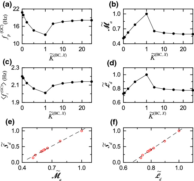
Quantitative relationship between sparsely synchronized rhythm of the GCs and pattern separation in the combined case of simultaneously changing the normalized synaptic strengths ${\tilde{K}}^{(\mathrm{BC},\mathrm{MC})}$ and ${\tilde{K}}^{(\mathrm{BC},\mathrm{HIPP})}$. a Plot of the population frequency $f_p^{(GC)}$ of sparsely synchronized rhythm of the GCs versus ${\tilde{K}}^{(\mathrm{BC},\mathrm{X})}$ (X= MC or HIPP). b Plot of the normalized amplitude measure, ${\tilde{\mathcal{M}}}_a$ versus ${\tilde{K}}^{(\mathrm{BC},\mathrm{X})}$. c Plot of the population-averaged mean firing rate $⟨f_i⟩$ versus ${\tilde{K}}^{(\mathrm{BC},\mathrm{X})}$. d Plot of the normalized random-spike-skipping degree ${\tilde{\mathcal{L}}}_d$ versus ${\tilde{K}}^{(\mathrm{BC},\mathrm{X})}$. (e) Plot of the normalized pattern separation degree ${\tilde{\mathcal{S}}}_d$ versus ${\tilde{\mathcal{M}}}_a$. f Plot of the normalized pattern separation degree ${\tilde{\mathcal{S}}}_d$ versus ${\tilde{\mathcal{L}}}_d$. Dashed fitted lines are given in (e–f)

As ${\tilde{K}}^{(\mathrm{BC},\mathrm{X})}$ is decreased from 1, the disynaptic inhibition effect of the MCs becomes dominant and decreased (i.e., less exciting the BCs). Hence, the firing activity of the GCs is found to increase, which results in increase in both $f_p^{(\mathrm{GC})}$ and $⟨f_i^{(\mathrm{GC})}⟩$. On the other hand, with increasing ${\tilde{K}}^{(\mathrm{BC},\mathrm{X})}$ from 1, the disynaptic effect of the HIPP cells becomes dominant and increased (i.e, more disinhibiting the BCs). Therefore, the firing activity of the GCs is also found to increase, which leads to increase in both $f_p^{(\mathrm{GC})}$ and $⟨f_i^{(\mathrm{GC})}⟩$.

We characterize the (population) synchronization degree of the sparsely synchronized rhythm of the GCs in terms of the amplitude measure ${\mathcal{M}}_a$, given by the time-averaged amplitude of the IPSR $R_{\mathrm{GC}}(t)$ (Kim and Lim 2021c):

$$\begin{array}{c}\hfill {\mathcal{M}}_a=\overline{{\mathcal{A}}_i};{\mathcal{A}}_i=\frac{[R_{\mathrm{GC},\max }^{(i)}(t)-R_{\mathrm{GC},\min }^{(i)}(t)]}{2},\end{array}$$ 19

where the overline represents time average, and $R_{\mathrm{GC},\max }^{(i)}(t)$ and $R_{\mathrm{GC},\min }^{(i)}(t)$ are the maximum and the minimum of $R_{\mathrm{GC}}(t)$ in its ith global cycle (corresponding to the ith spiking stripe), respectively. As ${\mathcal{M}}_a$ increases (i.e., the time-averaged amplitude of $R_{\mathrm{GC}}(t)$ is increased), the synchronization degree of the sparsely synchronized becomes higher.

Figure 6b shows the plot of the normalized amplitude measure ${\tilde{\mathcal{M}}}_a$ (= ${\mathcal{M}}_a/{\mathcal{M}}_a^{\ast }$) versus ${\tilde{K}}^{(\mathrm{BC},\mathrm{X})}$; ${\mathcal{M}}_a^{\ast }$ (= 3.566) is the default value for ${\tilde{K}}^{(\mathrm{BC},\mathrm{X})}=1$. We note that the normalized amplitude measure ${\tilde{\mathcal{M}}}_a$ is found to form a bell-shaped curve with an optimal maximum at the default value ${\tilde{K}}^{(\mathrm{BC},\mathrm{X})}=1$. As ${\tilde{K}}^{(\mathrm{BC},\mathrm{X})}$ is decreased from 1, ${\tilde{\mathcal{M}}}_a$ is decreased from 1 to 0.510, because the disynaptic inhibition effect of the MCs becomes dominant and decreased. Also, with increasing ${\tilde{K}}^{(\mathrm{BC},\mathrm{X})}$ from 1, ${\tilde{\mathcal{M}}}_a$ is also decreased from 1 and becomes saturated to 0.592 for ${\tilde{K}}^{(\mathrm{BC},\mathrm{X})}\sim 20$, because the disynaptic effect of the HIPP cells becomes dominant and increased.

Next, we characterize the individual spiking behavior of the active GCs in the ISI histogram with multiple peaks resulting from random spike skipping. We introduced a new random phase-locking degree ${\mathcal{L}}_d$, denoting how well intermittent spikes make phase-locking to $R_{\mathrm{GC}}(t)$ at random multiples of its global period $T_G^{(\mathrm{GC})}$ (Kim and Lim 2021d), and characterize the degree of random spike skipping seen in the ISI histogram in terms of ${\mathcal{L}}_d$. By following the approach developed in the case of pacing degree between spikes in the stripes in the raster plot of spikes (Kim and Lim 2014), the random phase-locking degree was introduced to examine the regularity of individual firings (represented well in the sharpness of the random-spike-skipping peaks).

We first locate the random-spike-skipping peaks in the ISI histogram. For each nth-order peak, we get the normalized weight $w_n$, given by:

$$\begin{array}{c}\hfill w_n=\frac{N_{\mathrm{ISI}}^{(n)}}{N_{\mathrm{ISI}}^{(tot)}},\end{array}$$ 20

where $N_{\mathrm{ISI}}^{(tot)}$ is the total number of ISIs obtained during the stimulus period ($T_s$ $=3·{10}^4$ msec) and $N_{\mathrm{ISI}}^{(n)}$ is the number of the ISIs in the nth-order peak.

We now consider the sequence of the ISIs, $\{{\mathrm{ISI}}_i^{(n)},i=1,\cdots ,N_{\mathrm{ISI}}^{(n)}\}$, within the nth-order peak, and get the random phase-locking degree ${\mathcal{L}}_d^{(n)}$ of the nth-order peak. Similar to the case of the pacing degree between spikes (Kim and Lim 2014), we provide a phase $\psi$ to each ${\mathrm{ISI}}_i^{(n)}$ via linear interpolation; for details, refer to (Kim and Lim 2021d). Then, the contribution of the ${\mathrm{ISI}}_i^{(n)}$ to the locking degree ${\mathcal{L}}_d^{(n)}$ is given by $cos({\psi }_i^{(n)})$; ${\psi }_i^{(n)}$ denotes the phase for ${\mathrm{ISI}}_i^{(n)}$. An ${\mathrm{ISI}}_i^{(n)}$ makes the most constructive contribution to ${\mathcal{L}}_d^{(n)}$ for ${\psi }_i^{(n)}=0$, while it makes no contribution to ${\mathcal{L}}_d^{(n)}$ for $\psi =\frac{\pi }{2}$ or $-\frac{\pi }{2}$. By averaging the matching contributions of all the ISIs in the nth-order peak, we get:

$$\begin{array}{c}\hfill {\mathcal{L}}_d^{(n)}=\frac{1}{N_{\mathrm{ISI}}^{(n)}}\sum _i^{N_{\mathrm{ISI}}^{(n)}}cos({\psi }_i^{(n)}).\end{array}$$ 21

Then, we obtain the (overall) random phase-locking degree ${\mathcal{L}}_d$ via weighted average of the random phase-locking degrees ${\mathcal{L}}_d^{(n)}$ of all the peaks:

$$\begin{array}{c}\hfill {\mathcal{L}}_d=\sum _{n=1}^{N_p}{w}_n·{\mathcal{L}}_d^{(n)}=\frac{1}{N_{\mathrm{ISI}}^{(\mathrm{tot})}}\sum _{n=1}^{N_p}\sum _{i=1}^{N_{\mathrm{ISI}}^{(\mathrm{tot})}}cos({\psi }_i^{(n)}),\end{array}$$ 22

where $N_p$ is the number of peaks in the ISI histogram. Thus, ${\mathcal{L}}_d$ corresponds to the average of contributions of all the ISIs in the ISI histogram.

Figure 6d shows the plot of the normalized random phase-locking degree ${\tilde{\mathcal{L}}}_d$ (=${\mathcal{L}}_d/{\mathcal{L}}_d^{\ast }$) versus ${\tilde{K}}^{(\mathrm{BC},\mathrm{X})}$; ${\mathcal{L}}_d^{\ast }$ (= 0.911) is the default value for ${\tilde{K}}^{(\mathrm{BC},\mathrm{X})}=1$. We note that the normalized random phase-locking degree ${\tilde{\mathcal{L}}}_d$ is found to form a bell-shaped curve with an optimal maximum at the default value of ${\tilde{K}}^{(\mathrm{BC},\mathrm{X})}=1$. In the default case, the random phase-locking degree ${\mathcal{L}}_d^{\ast }(=0.911)$, characterizing the sharpness of all the peaks, is the highest. Hence, the GCs make intermittent spikes which are well phase-locked to $R_{\mathrm{GC}}(t)$ at random multiples of its global period $T_G^{(\mathrm{GC})}$. However, with decreasing ${\tilde{K}}^{(\mathrm{BC},\mathrm{X})}$ from 1, ${\tilde{\mathcal{L}}}_d$ is decreased from 1 to 0.726, because the decreased disynaptic inhibition effect of the MCs becomes dominant. Also, as ${\tilde{K}}^{(\mathrm{BC},\mathrm{X})}$ is increased from 1, ${\tilde{\mathcal{L}}}_d$ is decreased from 1 and becomes saturated to 0.775 for ${\tilde{K}}^{(\mathrm{BC},\mathrm{X})}\sim 20$, because the increased disynaptic effect of the HIPP cells becomes dominant.

Finally, we investigate quantitative association between sparsely synchronized rhythm and pattern separation. Figure 6e and f show plots of ${\tilde{\mathcal{M}}}_a$ and ${\tilde{\mathcal{L}}}_d$ versus the normalized pattern separation degree ${\tilde{\mathcal{S}}}_d$, respectively. Population (${\tilde{\mathcal{M}}}_a$) and individual (${\tilde{\mathcal{L}}}_d$) firing behaviors in the sparsely synchronized rhythm of the GCs (performing pattern separation) are found to be positively correlated with the pattern separation (${\tilde{\mathcal{S}}}_d$) with the Pearson’s correlation coefficients $r=0.9959$ and 0.9975, respectively. Consequently, as ${\tilde{\mathcal{M}}}_a$ and ${\tilde{\mathcal{L}}}_d$ of the sparsely synchronized rhythm are larger, the pattern separation degree becomes higher; the better population and individual firing activities in the sparsely synchronized rhythm are, the more pattern separation efficacy becomes enhanced.

Summary and discussion

We considered the disynaptic paths from the hilar cells (i.e., excitatory MCs and inhibitory HIPP cells) to the principal excitatory GCs (performing pattern separation), mediated by the inhibitory BCs; MC $\to$ BC $\to$ GC and HIPP $\to$ BC $\to$ GC. We note that, disynaptic inhibition (mediated by the intermediate BCs) from the MCs decreases the activity of the GCs due to increased excitation of the BCs, while due to their disinhibition of the intermediate BCs, the disynaptic effect of the HIPP cells leads to increase in the activity of the GCs. In this way, their disynaptic effects on the GCs are opposite.

By changing the synaptic strength $K^{(\mathrm{BC},\mathrm{X})}$ [from the pre-synaptic X (= MC or HIPP) to the post-synaptic BC] from the original default value ${K^{(\mathrm{BC},\mathrm{X})}}^{\ast }$ in Table 2, we investigated the disynaptic effects of the MCs and the HIPP cells on the pattern separation (transforming the input patterns from the EC into sparser and orthogonalized output patterns) performed by the principal GCs. Here, we discuss their disynaptic effects by considering sparsity for the firing activity of the GCs which has been considered to improve the pattern separation. (Treves and Rolls 1994; O’Reilly and McClelland 1994; Schmidt et al. 2012; Rolls 2016; Knierim and Neunuebel 2016; Myers and Scharfman 2009, 2011; Myers et al. 2013; Scharfman and Myers 2016; Chavlis et al. 2017; Kassab and Alexandre 2018). Then, the pattern-separated output patterns are projected to the pyramidal cells in the CA3 subregion, which facilitates pattern storage and retrieval in the CA3. In this way, the DG plays a role of preprocessor for the CA3.

We first studied the disynaptic effect of the MCs by varying the normalized synaptic strength ${\tilde{K}}^{(\mathrm{BC},\mathrm{MC})}$ [= $K^{(\mathrm{BC},\mathrm{MC})}/{K^{(\mathrm{BC},\mathrm{MC})}}^{\ast }$]; ${K^{(\mathrm{BC},\mathrm{MC})}}^{\ast }$ is the original default value in Table 2. When ${\tilde{K}}^{(\mathrm{BC},\mathrm{MC})}$ is decreased from 1 (i.e., default value) to 0, excitation of the BCs decreases, which results in increase in the activation degree $D_a^{(out)}$ of the GCs and decrease in the orthogonalization degree $O^{(out)}$ between the two output patterns (generated by the GCs). We note that $D_a^{(out)}$ and $O^{(out)}$ are negatively correlated; as the firing activity of the GCs is sparser (i.e., $D_a^{(out)}$ is decreased), the orthogonalization efficacy, $O^{(out)}$, becomes increased. Consequently, with decreasing ${\tilde{K}}^{(\mathrm{BC},\mathrm{MC})}$ from 1, due to decrease in the pattern distance $D_p^{(out)}$ (given by the ratio of $O^{(out)}$ to $D_a^{(out)}$), the normalized pattern separation degree ${\tilde{\mathcal{S}}}_d$ [= ${\mathcal{S}}_d/{\mathcal{S}}_d^{\ast }$] (${\mathcal{S}}_d^{\ast }$: pattern separation degree at the default value) was decreased from 1 to 0.108. We note that, in this case, decrease in ${\tilde{\mathcal{S}}}_d$ results from decreased disynaptic inhibition to the GCs (leading to increase in $D_a^{(out)}$). This kind of decrease in the efficacy of pattern separation was also found through ablation of MCs (Danielson et al. 2017).

In contrast, as ${\tilde{K}}^{(\mathrm{BC},\mathrm{MC})}$ is increased from 1, more disynaptic inhibition, mediated by the BCs, is provided to the GCs, which leads to decrease in $D_a^{(out)}$ and increase in $O^{(out)}$ (i.e., negative correlation between $D_a^{(out)}$ and $O^{(out)}$ ). Thus, with increasing ${\tilde{K}}^{(\mathrm{BC},\mathrm{MC})}$ from 1, because of increase in $D_p^{(out)}$ (resulting from decreased $D_a^{(out)}$ and increased $O^{(out)}$), the normalized pattern separation degree ${\tilde{\mathcal{S}}}_d$ began to increase from 1 and become saturated to ${\tilde{\mathcal{S}}}_d\simeq 1.767$ for ${\tilde{K}}^{(\mathrm{BC},\mathrm{MC})}\sim 10$.

Overall, in the whole range of ${\tilde{K}}^{(\mathrm{BC},\mathrm{MC})}$, as it is increased from 0, disynaptic inhibition provided to the GCs increases, which results in decrease in $D_a^{(out)}$ and increase in $O^{(out)}$. Thus, due to increase in $D_p^{(out)}$ (resulting from decreased $D_a^{(out)}$ and increased $O^{(out)}$), the normalized pattern separation degree ${\tilde{\mathcal{S}}}_d$ was found to increase from 0.108 and get saturated to 1.767 for ${\tilde{K}}^{(\mathrm{BC},\mathrm{MC})}\sim 10$ (see blue solid circles in Fig. 4e). We note that, in this case of the MCs, increased disynaptic inhibition to the GCs (resulting in decrease in $D_a^{(out)}$) leads to increase in ${\tilde{\mathcal{S}}}_d$. Thus, sparsity for the firing activity of the GCs was found to improve the efficacy of pattern separation.

Next, we studied the disynaptic effect of the HIPP cells by varying the normalized synaptic strength ${\tilde{K}}^{(\mathrm{BC},\mathrm{HIPP})}$. The HIPP cells disinhibit the BCs, in contrast to the case of the MCs enhancing the activity of the BCs. Hence, the disynaptic effect of the HIPP cells on the pattern separation was found to be opposite to that of the MCs. Overall, as ${\tilde{K}}^{(\mathrm{BC},\mathrm{HIPP})}$ is increased from 0, BCs are more disinhibited, which leads to increase in $D_a^{(out)}$ and decrease in $O^{(out)}$. Hence, due to decrease in $D_p^{(out)}$ (resulting from increased $D_a^{(out)}$ and decreased $O^{(out)}$), the normalized pattern separation degree ${\tilde{\mathcal{S}}}_d$ was found to decrease from 2.819 and get saturated to 0.176 for ${\tilde{K}}^{(\mathrm{BC},\mathrm{HIPP})}\sim 20$ (see red open circles Fig. 4e). In this case of the HIPP cells, we note that, increased disinhibition of the BCs (leading to increase in $D_a^{(out)}$) results in decrease in ${\tilde{\mathcal{S}}}_d$, in contrast to the case of the MCs. Thus, increased firing activity of the GCs was found to worsen the pattern separation efficacy.

As a 3rd step, we considered the combined case when the two normalized synaptic strengths ${\tilde{K}}^{(\mathrm{BC},\mathrm{MC})}$ and ${\tilde{K}}^{(\mathrm{BC},\mathrm{HIPP})}$ were changed simultaneously. As a result of balance between the competing disynaptic effects of the MCs and the HIPP cells, the normalized pattern separation degree ${\tilde{\mathcal{S}}}_d$ was found to form a bell-shaped curve with an optimal maximum at the default value (i.e., ${\tilde{K}}^{(\mathrm{BC},\mathrm{MC})}={\tilde{K}}^{(\mathrm{BC},\mathrm{HIPP})}=1$) (see green crosses Fig. 4e); at the default value where the firing activity of the GCs is the sparest, the efficacy of pattern separation becomes the highest.

We note that, while the GCs perform pattern separation, sparsely synchronized rhythm was found to appear in the population of the GCs (see Fig. 5). We investigated quantitative association between population and individual firing behaviors in the sparsely synchronized rhythm and pattern separation. Population synchronization behavior and individual firing activities were characterized by employing the amplitude measure ${\mathcal{M}}_a$ (representing population synchronization degree) and the random-phase-locking degree ${\mathcal{L}}_d$ (denoting regularity degree of individual intermittent spikings), respectively. Both of them, ${\mathcal{M}}_a$ and ${\mathcal{L}}_d$, were found to be strongly correlated with the pattern separation degree ${\mathcal{S}}_d$ (see Fig. 6e and f). Hence, the larger ${\mathcal{M}}_a$ and ${\mathcal{L}}_d$ of the sparsely synchronized rhythm are, the more the pattern separation efficacy becomes enhanced.

For comparison, we also studied the monosynaptic effect of the MCs and the HIPP cells; MC $\to$ GC and HIPP $\to$ GC. Unlike the disynaptic case, the MCs and the HIPP cells provide direct excitation and inhibition to the GCs, respectively. Figure 7a, b, and c show the plots of the normalized average activation degree ${\tilde{D}}_a^{(out)}$ of the GCs, the normalized average orthogonalization degree ${\tilde{O}}^{(out)},$ and the normalized pattern separation degree ${\tilde{\mathcal{S}}}_d$ versus the normalized synaptic strength ${\tilde{K}}^{(\mathrm{GC},\mathrm{X})}$ [X= MC (blue solid circles) or HIPP (red open circles)], respectively. Here, the normalized synaptic strength ${\tilde{K}}_R^{(\mathrm{GC},\mathrm{X})}$ is given by $K_R^{(\mathrm{GC},\mathrm{X})}/{K_R^{(\mathrm{GC},\mathrm{X})}}^{\ast }$ ($\mathrm{X}=$ MC or HIPP and $R=$ AMPA, NMDA, or GABA), and ${K_R^{(\mathrm{GC},\mathrm{X})}}^{\ast }$ is the original default value in Table 1; ${K_{\mathrm{AMPA}}^{(\mathrm{GC},\mathrm{MC})}}^{\ast }=0.05$, ${K_{\mathrm{NMDA}}^{(\mathrm{GC},\mathrm{MC})}}^{\ast }=0.01,$ and ${K_{\mathrm{GABA}}^{(\mathrm{GC},\mathrm{HIPP})}}^{\ast }=0.13$. In the case of the MCs, we change ${\tilde{K}}_{\mathrm{AMPA}}^{(\mathrm{GC},\mathrm{MC})}$ and ${\tilde{K}}_{\mathrm{NMDA}}^{(\mathrm{GC},\mathrm{MC})}$ in the same way such that ${\tilde{K}}_{\mathrm{AMPA}}^{(\mathrm{GC},\mathrm{MC})}={\tilde{K}}_{\mathrm{NMDA}}^{(\mathrm{GC},\mathrm{MC})}\equiv {\tilde{K}}^{(\mathrm{GC},\mathrm{MC})}$, and in the case of the HIPP cells, for brevity, we write ${\tilde{K}}_{\mathrm{GABA}}^{(\mathrm{GC},\mathrm{HIPP})}$ as ${\tilde{K}}^{(\mathrm{GC},\mathrm{HIPP})}$.

Fig. 7.

Monosynaptic effect of the MCs and the HIPP cells on pattern separation. Plots of a the normalized average activation degree ${\tilde{D}}_a^{(out)},$ d b the normalized average orthogonalization degree ${\tilde{O}}^{(out)},$ and c the normalized pattern separation degree ${\tilde{\mathcal{S}}}_d$ versus the normalized synaptic strength ${\tilde{K}}^{(\mathrm{GC},\mathrm{X})}$ (X= MC or HIPP) for the output patterns. In a, b and c, solid circles, open circles, and crosses represent the cases of the MCs and the HIPP cells and the combined case, respectively. For clear presentation, we choose four different scales around (1, 1); (left, right) and (up, down)

In the whole range of ${\tilde{K}}^{(\mathrm{GC},\mathrm{X})}$, ${\tilde{D}}_a^{(out)}$, ${\tilde{O}}^{(out)},$ and ${\tilde{\mathcal{S}}}_d$ in the monosynaptic case show oppositely-changing tendencies, in comparison to those in the disynaptic case in Fig. 4, because the innervation effect on the GCs in the monosynaptic case is in opposition to that in the disynaptic case. In this monosynaptic case, ${\tilde{D}}_a^{(out)}$ and ${\tilde{O}}^{(out)}$ were also found to be negatively correlated (compare Fig. 7a with Fig. 7b). Particularly, in the combined case (see green crosses in Fig. 7) for simultaneous change in both ${\tilde{K}}^{(\mathrm{GC},\mathrm{MC})}$ and ${\tilde{K}}^{(\mathrm{GC},\mathrm{HIPP})}$, the normalized pattern separation degree ${\tilde{\mathcal{S}}}_d$ was found to form a well-shaped curve with an optimal minimum at the original default value (where the activation degree of the GCs is the highest), in contrast to disynaptic case with a bell-shaped curve for ${\tilde{\mathcal{S}}}_d$ with an optimal maximum at the default value (where the activation degree of the GCs are the lowest). Consequently, the pattern separation degree in the monosynaptic case becomes the lowest at the original default value, in opposition to the disynaptic case (with the highest pattern separation degree at the default value). However, in our DG network, disynaptic strengths are stronger than monosynaptic strengths (see Tables 1 and 2). Hence, when considering both the disynaptic and the monosynaptic effects simultaneously, the disynaptic effect becomes dominant (i.e., at the original default values, the normalized pattern separation degree becomes the highest).

Finally, we discuss limitations of our present work and future works. In the present work, although positive correlation between the pattern separation degree and the population synchronization and the random-phase-locking degrees in the sparsely synchronized rhythm of the GCs was found, this kind of correlation does not imply causal relationship. Hence, in future work, it would be interesting to make intensive investigation on their dynamical causation.

Also, in the present work, we studied disynaptic effect only in the case of changing the synaptic strength $K^{(\mathrm{BC},\mathrm{X})}$ (X= MC or HIPP). However, in future, it would also be interesting to study disynaptic effect by varying the connection probability $p^{(\mathrm{BC},\mathrm{X})}$ from the presynaptic X to the postsynaptic BC. The effect of decrease in $p^{(\mathrm{BC},\mathrm{X})}$ would be similar to that of decreasing $K^{(\mathrm{BC},\mathrm{X})}$, because the synaptic inputs into the BCs are decreased in both cases.

Furthermore, we note that the pyramidal cells in the CA3 provide backprojections to the GCs via polysynaptic connections (Myers and Scharfman 2011; Myers et al. 2013; Scharfman and Myers 2016). For example, the pyramidal cells send disynaptic inhibition to the GCs, mediated by the BCs and the HIPP cells in the DG, and they provide trisynaptic inputs to the GCs, mediated by the MCs (pyramidal cells $\to$ MC $\to$ BC or HIPP $\to$ GC). These inhibitory backprojections may decrease the activation degree of the GCs, leading to improvement of pattern separation. Hence, in future work, it would be meaningful to take into consideration the backprojection for the study of pattern separation in the combined DG-CA3 network.

Also, in the present study, for simplicity, we did not consider the lamellar organization for the hilar MCs and the HIPP cells, as in (Myers and Scharfman 2009; Chavlis et al. 2017); here, we considered only the GC lamellar clusters. For more refined DG network, it would be necessary in future work to take into consideration the lamellar organization for the MCs and the HIPP cells; particularly, in the combined DG-CA3 network for pattern storage and retrieval, as in (Myers and Scharfman 2011; Myers et al. 2013; Scharfman and Myers 2016).

References

- Almeida LD, Idiart M, Lisman JE. A second function of gamma frequency oscillations: An E%-max winner-take-all mechanism selects which cells fire. J Neurosci. 2009;29:7497–7503. doi: 10.1523/JNEUROSCI.6044-08.2009. [DOI] [PMC free article] [PubMed] [Google Scholar]
- Amaral DG, Witter MP. The three-dimensional organization of the hippocampal formation: A review of anatomical data. Neuroscience. 1989;31:571–591. doi: 10.1016/0306-4522(89)90424-7. [DOI] [PubMed] [Google Scholar]
- Amaral DG, Ishizuka N, Claiborne B. Neurons, numbers and the hippocampal network. Prog Brain Res. 1990;83:1–11. doi: 10.1016/s0079-6123(08)61237-6. [DOI] [PubMed] [Google Scholar]
- Amaral DG, Scharfman HE, Lavenex P. The dentate gyrus: fundamental neuroanatomical organization (dentate gyrus for dummies) Prog Brain Res. 2007;163:3–22. doi: 10.1016/S0079-6123(07)63001-5. [DOI] [PMC free article] [PubMed] [Google Scholar]
- Andersen P, Bliss TVP, Skrede KK. Lamellar organization of hippocampal excitatory pathways. Exp Brain Res. 1971;13:222–238. doi: 10.1007/BF00234087. [DOI] [PubMed] [Google Scholar]
- Andersen P, Soleng AF, Raastad M. The hippocampal lamella hypothesis revisited. Brain Res. 2000;886:165–171. doi: 10.1016/s0006-8993(00)02991-7. [DOI] [PubMed] [Google Scholar]
- Bakker A, Kirwan CB, Miller M, Stark CEL. Pattern separation in the human hippocampal CA3 and dentate gyrus. Science. 2008;319:1640–1642. doi: 10.1126/science.1152882. [DOI] [PMC free article] [PubMed] [Google Scholar]
- Barranca VJ, Huang H, Kawakita G. Network structure and input integration in competing firing rate models for decision-making. J Comput Neurosci. 2019;46:145–168. doi: 10.1007/s10827-018-0708-6. [DOI] [PubMed] [Google Scholar]
- Bartos M, Vida I, Frotscher M, Geiger JR, Jonas P. Rapid signaling at inhibitory synapses in a dentate gyrus interneuron network. J Neurosci. 2001;21:2687–2698. doi: 10.1523/JNEUROSCI.21-08-02687.2001. [DOI] [PMC free article] [PubMed] [Google Scholar]
- Beck H, Goussakov IV, Lie A, Helmstaedter C, Elger CE. Synaptic plasticity in the human dentate gyrus. J Neurosci. 2000;20:7080–7086. doi: 10.1523/JNEUROSCI.20-18-07080.2000. [DOI] [PMC free article] [PubMed] [Google Scholar]
- Bielczyk NZ, Piskała K, Płomecka M, Radziński P, Todorova L, Foryś U. Time-delay model of perceptual decision making in cortical networks. PLoS One. 2019;14:e0211885. doi: 10.1371/journal.pone.0211885. [DOI] [PMC free article] [PubMed] [Google Scholar]
- Brunel N, Hakim V. Sparsely synchronized neuronal oscillations. Chaos. 2008;18:015113. doi: 10.1063/1.2779858. [DOI] [PubMed] [Google Scholar]
- Brunel N, Wang XJ. What determines the frequency of fast network oscillations with irregular neural discharges? I. Synaptic dynamics and excitation-inhibition balance. J Neurophysiol. 2003;90:415–430. doi: 10.1152/jn.01095.2002. [DOI] [PubMed] [Google Scholar]
- Buckmaster PS, Jongen-Rêlo AL. Highly specific neuron loss preserves lateral inhibitory circuits in the dentate gyrus of kainite-induced epileptic rats. J Neurosci. 1999;19:9519–9529. doi: 10.1523/JNEUROSCI.19-21-09519.1999. [DOI] [PMC free article] [PubMed] [Google Scholar]
- Buckmaster PS, Wenzel HJ, Kunkel DD, Schwartzkroin PA. Axon arbors and synaptic connections of hippocampal mossy cells in the rat in vivo. J Comp Neurol. 1996;366:271–292. doi: 10.1002/(sici)1096-9861(19960304)366:2<270::aid-cne7>3.0.co;2-2. [DOI] [PubMed] [Google Scholar]
- Buckmaster PS, Yamawaki R, Zhang GF. Axon arbors and synaptic connections of a vulnerable population of interneurons in the dentate gyrus in vivo. J Comp Neurol. 2002;445:360–373. doi: 10.1002/cne.10183. [DOI] [PubMed] [Google Scholar]
- Chavlis S, Petrantonakis PC, Poirazi P. Dendrites of dentate gyrus granule cells contribute to pattern separation by controlling sparsity. Hippocampus. 2017;27:89–110. doi: 10.1002/hipo.22675. [DOI] [PMC free article] [PubMed] [Google Scholar]
- Chiang PH, Wu PY, Kuo TW, Liu YC, Chan CF, Chien TC, Cheng JK, Huang YY, Chiu CD, Lien CC. GABA is depolarizing in hippocampal dentate granule cells of the adolescent and adult rats. J Neurosci. 2012;32:62–67. doi: 10.1523/JNEUROSCI.3393-11.2012. [DOI] [PMC free article] [PubMed] [Google Scholar]
- Coultrip R, Granger R, Lynch G. A cortical model of winner-take-all competition via lateral inhibition. Neural Netw. 1992;5:47–54. [Google Scholar]
- Danielson NB, Turi GF, Ladow M, Chavlis S, Petrantonakis PC, Poirazi P, Losonczy A. In vivo imaging of dentate gyrus mossy cells in behaving mice. Neuron. 2017;93:552–559. doi: 10.1016/j.neuron.2016.12.019. [DOI] [PMC free article] [PubMed] [Google Scholar]
- van Dijk MT, Fenton AA. On how the dentate gyrus contributes to memory discrimination. Neuron. 2018;98:832–845. doi: 10.1016/j.neuron.2018.04.018. [DOI] [PMC free article] [PubMed] [Google Scholar]
- Dudek SM, Alexander GM, Farris S. Rediscovering area CA2: unique properties and functions. Nat Rev Nurosci. 2016;17:89–102. doi: 10.1038/nrn.2015.22. [DOI] [PMC free article] [PubMed] [Google Scholar]
- Espinoza C, Guzman SJ, Zhang X, Jonas P. Parvalbumin+ interneurons obey unique connectivity rules and establish a powerful lateral inhibition microcircuit in dentate gyrus. Nat Commun. 2018;9:4605. doi: 10.1038/s41467-018-06899-3. [DOI] [PMC free article] [PubMed] [Google Scholar]
- Geiger JRP, Lübke J, Roth A, Frotscher M, Jonas P. Submillisecond AMPA receptor-mediated signaling at a principal neuron-interneuron synapse. Neuron. 1997;18:1009–1023. doi: 10.1016/s0896-6273(00)80339-6. [DOI] [PubMed] [Google Scholar]
- Geisler C, Brunel N, Wang XJ. Contributions of intrinsic membrane dynamics to fast network oscillations with irregular neuronal discharges. J Neurophysiol. 2005;94:4344–4361. doi: 10.1152/jn.00510.2004. [DOI] [PubMed] [Google Scholar]
- Gerstner W, Kistler W. Spiking Neuron Models. New York: Cambridge University Press; 2002. [Google Scholar]
- Gluck MA, Myers CE. Gateway to Memory: An Introduction to Neural Network Modeling of the Hippocampus in Learning and Memory. Cambridge: MIT Press; 2001. [Google Scholar]
- Hafting T, Fyhn M, Molden S, Moser MB, Moser EI. Microstructure of a spatial map in the entorhinal cortex. Nature. 2005;436:801–806. doi: 10.1038/nature03721. [DOI] [PubMed] [Google Scholar]
- Hosp JA, Strüber M, Yanagawa Y, Obata K, Vida I, Jonas P, Bartos M. Morpho-physiological criteria divide dentate gyrus interneurons into classes. Hippocampus. 2014;24:189–203. doi: 10.1002/hipo.22214. [DOI] [PMC free article] [PubMed] [Google Scholar]
- Houghton C. Dentate gyrus and hilar region revisited. Behav Brain Sci. 2017;39:28–29. doi: 10.1017/S0140525X15001818. [DOI] [PubMed] [Google Scholar]
- Hsu TT, Lee CT, Tai MH, Lien CC. Differential recruitment of dentate gyrus interneuron types by commissural versus performant pathways. Cerebral Cortex. 2016;26:2715–2727. doi: 10.1093/cercor/bhv127. [DOI] [PubMed] [Google Scholar]
- Jahr CE, Stevens CF. Voltage dependence of NMDA-activated macroscopic conductances predicted by single-channel kinetics. J Neurosci. 1990;10:3178–3182. doi: 10.1523/JNEUROSCI.10-09-03178.1990. [DOI] [PMC free article] [PubMed] [Google Scholar]
- Jinde S, Zsiros V, Jiang Z, Nakao K, Pickel J, Kohno K, Belforte JE, Nakazawa K. Hilar mossy cell degeneration causes transient dentate granule cell hyperexcitability and impaired pattern separation. Neuron. 2012;76:1189–1200. doi: 10.1016/j.neuron.2012.10.036. [DOI] [PMC free article] [PubMed] [Google Scholar]
- Jinde S, Zsiros V, Nakazawa K. Hilar mossy cell circuitry controlling dentate granule cell excitability. Front Neural Circuit. 2013;7:14. doi: 10.3389/fncir.2013.00014. [DOI] [PMC free article] [PubMed] [Google Scholar]
- Kassab R, Alexandre F. Pattern separation in the hippocampus: distinct circuits under different conditions. Brain Struct Funct. 2018;223:2785–2808. doi: 10.1007/s00429-018-1659-4. [DOI] [PubMed] [Google Scholar]
- Kim SY, Lim W. Realistic thermodynamic and statistical-mechanical measures for neural synchronization. J Neurosci Meth. 2014;226:161–170. doi: 10.1016/j.jneumeth.2013.12.013. [DOI] [PubMed] [Google Scholar]
- Kim SY, Lim W. Effect of inhibitory spike-timing-dependent plasticity on fast sparsely synchronized rhythms in a small-world neuronal network. Neural Netw. 2018;106:50–66. doi: 10.1016/j.neunet.2018.06.013. [DOI] [PubMed] [Google Scholar]
- Kim SY, Lim W. Effect of diverse recoding of granule cells on optokinetic response in a cerebellar ring network with synaptic plasticity. Neural Netw. 2021;134:173–204. doi: 10.1016/j.neunet.2020.11.014. [DOI] [PubMed] [Google Scholar]
- Kim SY, Lim W. Influence of various temporal recoding on Pavlovian eyeblink conditioning in the cerebellum. Cogn Neurodyn. 2021;15:1067–1099. doi: 10.1007/s11571-021-09673-2. [DOI] [PMC free article] [PubMed] [Google Scholar]
- Kim SY, Lim W. Equalization effect in interpopulation spike-timing-dependent plasticity in two inhibitory and excitatory populations. In: Lintas A, Enrico P, Pan X, Wang R, Villa A, editors. Advances in Cognitive Neurodynamics (VII) Singapore: Springer; 2021. pp. 75–82. [Google Scholar]
- Kim SY, Lim W. Population and individual firing behaviors in sparsely synchronixed rhythms in the hippocampal dentata gyrus. Cogn Neurodyn. 2021 doi: 10.1007/s11571-021-09728-4. [DOI] [PMC free article] [PubMed] [Google Scholar]
- Kim SY, Lim W (2022) Dynamical origin for winner-take-all competition in a biological network of the hippocampal dentate gyrus. Phys Rev E (Accepted for Publication) [DOI] [PubMed]
- Kneisler TB, Dingledine R. Spontaneous and synaptic input from granule cells and the perforant path to dentate basket cells in the rat hippocampus. Hippocampus. 1995;5:151–164. doi: 10.1002/hipo.450050302. [DOI] [PubMed] [Google Scholar]
- Knierim JJ, Neunuebel JP. Tracking the flow of hippocampal computation: Pattern separation, pattern completion, and attractor dynamics. Neurobiol Learn Mem. 2016;129:38–49. doi: 10.1016/j.nlm.2015.10.008. [DOI] [PMC free article] [PubMed] [Google Scholar]
- Krueppel R, Remy S, Beck H. Dendritic integration in hippocampal dentate granule cells. Neuron. 2011;71:512–528. doi: 10.1016/j.neuron.2011.05.043. [DOI] [PubMed] [Google Scholar]
- Larimer P, Strowbridge BW. Nonrandom local circuits in the dentate gyrus. J Neurosci. 2008;28:12212–12223. doi: 10.1523/JNEUROSCI.3612-08.2008. [DOI] [PMC free article] [PubMed] [Google Scholar]
- Leutgeb JK, Leutgeb S, Moser MB, Moser EI. Pattern separation in the dentate gyrus and CA3 of the hippocampus. Science. 2007;315:961–966. doi: 10.1126/science.1135801. [DOI] [PubMed] [Google Scholar]
- Liu YC, Cheng JK, Lien CC. Rapid dynamic changes of dendritic inhibition in the dentate gyrus by presynaptic activity patterns. J Neurosci. 2014;34:1344–1357. doi: 10.1523/JNEUROSCI.2566-13.2014. [DOI] [PMC free article] [PubMed] [Google Scholar]
- Lübke J, Frotscher M, Spruston N. Specialized electrophysiological properties of anatomically identified neurons in the hilar region of the rat fascia dentata. J Neurophysiol. 1998;79:1518–1534. doi: 10.1152/jn.1998.79.3.1518. [DOI] [PubMed] [Google Scholar]
- Marr D. Simple memory: A theory for archicortex. Phil Trans R Soc Lond B. 1971;262:23–81. doi: 10.1098/rstb.1971.0078. [DOI] [PubMed] [Google Scholar]
- McNaughton B, Morris R. Hippocampal synaptic enhancement and information storage within a distributed memory system. Trends Neurosci. 1987;10:408–415. [Google Scholar]
- McNaughton BL, Barnes CA, Mizumori SJY, Green EJ, Sharp PE. Contribution of granule cells to spatial representations in hippocampal circuits: A puzzle. In: Morrell F, editor. Kindling and Synaptic Plasticity: The Legacy of Graham Goddar. Boston: Springer-Verlag; 1991. pp. 110–123. [Google Scholar]
- Morgan RJ, Santhakumar V, Soletsz I. Modeling the dentate gyrus. Prog Brain Res. 2007;163:639–658. doi: 10.1016/S0079-6123(07)63035-0. [DOI] [PubMed] [Google Scholar]
- Myers CE, Scharfman HE. A role for hilar cells in pattern separation in the dentate gyrus: A computational approach. Hippocampus. 2009;19:321–337. doi: 10.1002/hipo.20516. [DOI] [PMC free article] [PubMed] [Google Scholar]
- Myers CE, Scharfman HE. Pattern separation in the dentate gyrus: A role for the CA3 backprojection. Hippocampus. 2011;21:1190–1215. doi: 10.1002/hipo.20828. [DOI] [PMC free article] [PubMed] [Google Scholar]
- Myers CE, Bermudez-Hernandez K, Scharfman HE. The influence of ectopic migration of granule cells into the hilus on dentate gyrus-CA3 function. PLoS ONE. 2013;8:e68208. doi: 10.1371/journal.pone.0068208. [DOI] [PMC free article] [PubMed] [Google Scholar]
- Nitz D, McNaughton B. Differential modulation of CA1 and dentate gyrus interneurons during exploration of novel environments. J Neurophysiol. 2004;91:863–872. doi: 10.1152/jn.00614.2003. [DOI] [PubMed] [Google Scholar]
- Nomura T, Fukuda T, Aika Y, Heizmann CW, Emson PC, Kobayashi T, Kosaka T. Distribution of nonprincipal neurons in the rat hippocampus, with special reference to their dorsoventral difference. Brain Res. 1997;751:64–80. doi: 10.1016/s0006-8993(96)01395-9. [DOI] [PubMed] [Google Scholar]
- Nomura T, Fukuda T, Aika Y, Heizmann CW, Emson PC, Kobayashi T, Kosaka T. Laminar distribution of non-principal neurons in the rat hippocampus, with special reference to their compositional difference among layers. Brain Res. 1997;764:197–204. doi: 10.1016/s0006-8993(97)00457-5. [DOI] [PubMed] [Google Scholar]
- O’Reilly RC, McClelland JC. Hippocampal conjunctive encoding, storage, and recall: Avoiding a tradeoff. Hippocampus. 1994;4:661–682. doi: 10.1002/hipo.450040605. [DOI] [PubMed] [Google Scholar]
- Petrantonakis PC, Poirazi P. A compressed sensing perspective of hippocampal function. Front Syst Neurosci. 2014;8:141. doi: 10.3389/fnsys.2014.00141. [DOI] [PMC free article] [PubMed] [Google Scholar]
- Petrantonakis PC, Poirazi P. Dentate gyrus circuitry features improve performance of sparse approximation algorithms. PLoS One. 2015;10:e0117023. doi: 10.1371/journal.pone.0117023. [DOI] [PMC free article] [PubMed] [Google Scholar]
- Ratzliff ADH, Howard AL, Santhakumar V, Osapay I, Soltesz I. Rapid deletion of mossy cells does not result in a hyperexcitable dentate gyrus: Implications for epileptogenesis. J Neurosci. 2004;24:2259–2269. doi: 10.1523/JNEUROSCI.5191-03.2004. [DOI] [PMC free article] [PubMed] [Google Scholar]
- Rolls ET. Functions of neuronal networks in the hippocampus and neocortex in memory. In: Byrne JH, Berry WO, editors. Neural Models of Plasticity: Experimental and Theoretical Approaches. San Diego: Academic Press; 1989. pp. 240–265. [Google Scholar]
- Rolls ET. The representation and storage of information in neural networks in the primate cerebral cortex and hippocampus. In: Durbin R, Miall C, Mitchison G, editors. The Computing Neuron. Wokingham: Addition-Wesley; 1989. pp. 125–159. [Google Scholar]
- Rolls ET. Functions of neuronal networks in the hippocampus and cerebral cortex in memory. In: Cotterill R, editor. Models of Brain Function. New York: Cambridge University Press; 1989. pp. 15–33. [Google Scholar]
- Rolls ET. Pattern separation, completion, and categorization in the hippocampus and neocortex. Neurobiol Learn Mem. 2016;129:4–28. doi: 10.1016/j.nlm.2015.07.008. [DOI] [PubMed] [Google Scholar]
- Santhakumar V, Aradi I, Soltesz I. Role of mossy fiber sprouting and mossy cell loss in hyperexcitability: A network model of the dentate gyrus incorporating cell types and axonal topography. J Neurophysiol. 2005;93:437–453. doi: 10.1152/jn.00777.2004. [DOI] [PubMed] [Google Scholar]
- Santoro A. Reassessing pattern separation in the dentate gyrus. Front Behav Neurosci. 2013;7:96. doi: 10.3389/fnbeh.2013.00096. [DOI] [PMC free article] [PubMed] [Google Scholar]
- Savanthrapadian S, Meyer T, Elgueta C, Booker SA, Vida I, Bartos M. Synaptic properties of SOM- and CCK-expressing cells in dentate gyrus interneuron networks. J Neurosci. 2014;34:8197–8209. doi: 10.1523/JNEUROSCI.5433-13.2014. [DOI] [PMC free article] [PubMed] [Google Scholar]
- Scharfman HE. Dentate hilar cells with dendrites in the molecular layer have lower thresholds for synaptic activation by perforant path than granule cells. J Neurosci. 1991;11:1660–1673. doi: 10.1523/JNEUROSCI.11-06-01660.1991. [DOI] [PMC free article] [PubMed] [Google Scholar]
- Scharfman HE. Advances in understanding hilar mossy cells of the dentate gyrus. Cell Tissue Res. 2018;373:643–652. doi: 10.1007/s00441-017-2750-5. [DOI] [PMC free article] [PubMed] [Google Scholar]
- Scharfman HE, Myers CE. Hilar mossy cells of the dentate gyrus: A historical perspective. Front Neural Circuit. 2013;6:106. doi: 10.3389/fncir.2012.00106. [DOI] [PMC free article] [PubMed] [Google Scholar]
- Scharfman HE, Myers CE. Corruption of the dentate gyrus by “dominant” granule cells: Implications for dentate gyrus function in health and disease. Neurobiol Learn Mem. 2016;129:69–82. doi: 10.1016/j.nlm.2015.09.005. [DOI] [PMC free article] [PubMed] [Google Scholar]
- Schmidt B, Marrone DF, Markus EJ. Disambiguating the similar: The dentate gyrus and pattern separation. Behav Brain Res. 2012;226:56–65. doi: 10.1016/j.bbr.2011.08.039. [DOI] [PubMed] [Google Scholar]
- Schmidt-Hieber C, Bischofberger J. Fast sodium channel gating supports localized and efficient axonal action potential initiation. J Neurosci. 2010;30:10233–10242. doi: 10.1523/JNEUROSCI.6335-09.2010. [DOI] [PMC free article] [PubMed] [Google Scholar]
- Schmidt-Hieber C, Jonas P, Bischofberger J. Subthreshold dendritic signal processing and coincidence detection in dentate gyrus granule cells. J Neurosci. 2007;27:8430–8441. doi: 10.1523/JNEUROSCI.1787-07.2007. [DOI] [PMC free article] [PubMed] [Google Scholar]
- Shimazaki H, Shinomoto S. Kernel bandwidth optimization in spike rate estimation. J Comput Neurosci. 2010;29:171–182. doi: 10.1007/s10827-009-0180-4. [DOI] [PMC free article] [PubMed] [Google Scholar]
- Sloviter RS, Lømo T. Updating the lamellar hypothesis of hippocampal organization. Front Neural Circuit. 2012;6:102. doi: 10.3389/fncir.2012.00102. [DOI] [PMC free article] [PubMed] [Google Scholar]
- Squire L. Memory and Brain. New York: Oxford University Press; 1987. [Google Scholar]
- Su L, Chang CJ, Lynch N. Spike-based winner-take-all computation: Fundamental limits and order-optimal circuits. Neural Comput. 2019;31:2523–2561. doi: 10.1162/neco_a_01242. [DOI] [PubMed] [Google Scholar]
- Treves A, Rolls ET. What determines the capacity of autoassociative memories in the brain? Network. 1991;2:371–397. [Google Scholar]
- Treves A, Rolls ET. Computational constraints suggest the need for two distinct input systems to the hippocampal CA3 network. Hippocampus. 1992;2:189–199. doi: 10.1002/hipo.450020209. [DOI] [PubMed] [Google Scholar]
- Treves A, Rolls ET. Computational analysis of the role of the hippocampus in memory. Hippocampus. 1994;4:374–391. doi: 10.1002/hipo.450040319. [DOI] [PubMed] [Google Scholar]
- Wang XJ. Neurophysiological and computational principles of fscortical rhythms in cognition. Physiol Rev. 2010;90:1195–1268. doi: 10.1152/physrev.00035.2008. [DOI] [PMC free article] [PubMed] [Google Scholar]
- Wang Y, Zhang X, Xin Q, Hung W, Florman J, Huo J, Xu T, Xie Y, Alkema MJ, Zhen M, Wen Q. Flexible motor sequence generation during stereotyped escape responses. eLife. 2020;9:e56942. doi: 10.7554/eLife.56942. [DOI] [PMC free article] [PubMed] [Google Scholar]
- West MJ, Slomianka L, Gundersen HJ. Unbiased stereological estimation of the total number of neurons in the subdivisions of the rat hippocampus using the optical fractionator. Anat Rec. 1991;231:482–497. doi: 10.1002/ar.1092310411. [DOI] [PubMed] [Google Scholar]
- Willshaw D, Buckingham J. An assessment of Marr’s theory of the hippocampus as a temporary memory store. Phil Trans R Soc Lond B. 1990;329:205–215. doi: 10.1098/rstb.1990.0165. [DOI] [PubMed] [Google Scholar]
- Yassa MA, Stark CEL. Pattern separation in the hippocampus. Trends Neurosci. 2011;34:515–525. doi: 10.1016/j.tins.2011.06.006. [DOI] [PMC free article] [PubMed] [Google Scholar]
- Yim MY, Hanuschkin A, Wolfart J. Intrinsic rescaling of granule cells restores pattern separation ability of a dentate gyrus network model during epileptic hyperexcitability. Hippocampus. 2015;25:297–308. doi: 10.1002/hipo.22373. [DOI] [PubMed] [Google Scholar]