Prospective contingency explains behavior and dopamine signals during associative learning

Abstract

Associative learning depends on contingency, the degree to which a stimulus predicts an outcome. Despite its importance, the neural mechanisms linking contingency to behavior remain elusive. Here we examined the dopamine activity in the ventral striatum – a signal implicated in associative learning – in a Pavlovian contingency degradation task in mice. We show that both anticipatory licking and dopamine responses to a conditioned stimulus decreased when additional rewards were delivered uncued, but remained unchanged if additional rewards were cued. These results conflict with contingency-based accounts using a traditional definition of contingency or a novel causal learning model (ANCCR), but can be explained by temporal difference (TD) learning models equipped with an appropriate inter-trial-interval (ITI) state representation. Recurrent neural networks trained within a TD framework develop state representations like our best ‘handcrafted’ model. Our findings suggest that the TD error can be a measure that describes both contingency and dopaminergic activity.

Introduction

Learning predictive relationships between events is crucial for adaptive behaviors. Early investigations showed contiguity between two events (“pairing”) is insufficient for association: when an initially neutral cue (conditioned stimulus, CS) is paired with an outcome (unconditioned stimulus, US), such as electric shock, an animal learns to respond to the CS, anticipating the outcome, e.g. freezing to CSs that predict shock. But if the shocks are delivered at the same rate regardless of the absence or presence of the CS, animals do not freeze to the CS¹. Moreover, if a CS predicts a decrease in the likelihood of the US, conditioned responding decreases. From this observation, Rescorla postulated conditioning depends not on contiguity, but contingency – the extent to which the CS signals a change in the likelihood of the US. Work in statistics and artificial intelligence suggest contingency may also be central to understanding causal inference.

Yet a good behaviorally meaningful measure of contingency remains elusive^2–5. A commonly adopted definition in psychology and causal inference is ΔP, the probability difference of one event occurring in the presence or absence of another^6,7. In Pavlovian settings with trial-like structures, like this study, $\Delta P=P\left(US\right|CS+)-P(US|CS-)$, with ‘CS+’ and ‘CS−’ indicating the CS presence/absence. Experimentally, $\mathrm{\Delta }\mathrm{P}$ correlates with perceived causal strength^4,8,9. Although $\mathrm{\Delta }\mathrm{P}$ is a straightforward definition, it does not incorporate temporal relationships, working well only for trial-like structures. Furthermore, some behavioral observations cannot be explained by $\Delta P$, leading some to argue against the usefulness of contingency in explaining behavior¹⁰ and others to propose more nuanced definitions^2–5.

Subsequent experiments emphasized the role of surprise in associative learning¹¹. Rescorla and Wagner postulated that conditioning is driven by the discrepancy between actual and predicted outcomes (prediction errors)¹². Importantly, their contiguity-based model can explain the freezing responses to cues of different contingency. To achieve this, the context is assumed to be another CS, competing with the primary CS. While an attractive account of these experiments, this ‘cue-competition’ model is contested by other work^13–15.

Like $\mathrm{\Delta }\mathrm{P}$, the Rescorla-Wagner model assumes a trial-based structure and neglects event timing. Addressing this limitation, Sutton and Barto developed the temporal difference (TD) learning algorithm, now a fundamental algorithm in reinforcement learning (RL)^16,17, as a prediction error-based model of associative learning. The striking resemblance between the prediction errors of this model (TD error) and the activity of midbrain dopamine neurons is used as evidence of TD learning as an explanation of associative learning^18–20.

Despite the successes of TD learning as an explanatory model^18,21, alternatives have been proposed to explain dopamine and behavior. Recently, a study²² proposed a model called adjusted net contingency for causal relations (ANCCR). As the name suggests, ANCCR posits contingency as central to associative learning and causal inference. While conventional definitions of contingency and TD learning models consider “prospective” predictive relationships between cues and outcomes, i.e. $P\left(US\right|CS)$, in ANCCR learning is driven by “retrospective” relationships, the probability of a stimulus given the outcome, or $P\left(CS\right|US)$. The authors argue ANCCR implements causal inference, and that dopamine signals convey a signal for causal learning (the “adjusted net contingency”), not TD errors, claiming this model succeeds and TD fails to explain dopamine signals in mice²² and rats²³ in Pavlovian experiments manipulating contingency.

Contingency lies at the heart of learning predictive relationships, though how this is instantiated in the brain and manifests in behavior remains unclear. To address this, we examined behavior and dopamine signals in the ventral striatum (VS) in mice performing Pavlovian conditioning tasks while manipulating stimulus-outcome contingencies. We show, contrary to previous claims^22,23, dopamine signals could be comprehensively explained by TD learning models with appropriate state space representation. Further, we found dopamine signals primarily reflected prospective stimulus-outcome relationships, strongly violating predictions of the ANCCR model. We then discuss a framework relating dopamine signals to contingency and causal inference.

Results

Contingency degradation attenuates Pavlovian conditioned responding

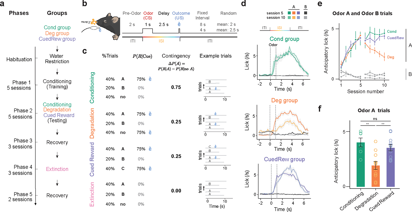
To study the effects of contingency in a Pavlovian setting, we developed a task for head-fixed mice where odor cues predicted a stochastic reward (Fig. 1a, b, c). Mice (n = 30) were first trained on one reward-predicting odor (Odor A) that predicted a reward (9 μL water) with 75% probability, and one odor (Odor B) that indicated no reward. In this phase (Phase 1), Odor A trials accounted for 40% of trials, Odor B for 20%, with the remaining 40% being blank trials, with no odor or reward delivered. The timing (Fig. 1b) was chosen such that the trial length was relatively constant allowing us to apply the classic $\mathrm{\Delta }P$ definition.

Figure 1.

Dynamic changes in lick response to olfactory cues across different phases of Pavlovian contingency learning task.

(a) Experimental design. Three groups of mice subjected to four unique conditions of contingency learning. All animals underwent Phases 1 and 2. Deg group additionally underwent Phases 3–5.

(b) Trial timing.

(c) Trial parameters per condition. In Conditioning, Degradation and Cued Reward, Odor A predicts 75% chance of reward (9 μL water) delivery, Odor B indicates no reward. In Degradation, blank trials were replaced with uncued rewards (75% reward probability). In Cued Reward, these additional rewards were cued by Odor C. In Extinction, no rewards were delivered.

(d) PSTH of average licking response of mice in three groups to the onset of Odor A and Odor B from the last session of Phase 1 (session 5) and Phase 2 (session 10). Shaded area is standard error of the mean (SEM). Notably, the decreased licking response during ISI and increased during ITI in Deg group. (green, Cond group, n = 6; orange, Deg group, n = 11; purple, CuedRew group, n = 12 mice).

(e) Average lick rate in 3s post-cue (Odor A or B) by session. Error bars represent SEM.

(f) Average lick rate in 3s post Odor A in final session of each condition. Asterisks denote statistical significance: ns, P > 0.05; **, P < 0.01, indicating a significant change in licking behavior to Odor A in Deg group across sessions using 2-sided mixed-effects model with Tukey’s HSD post-hoc tests (Cond vs CuedRew, p = 0.77; Cond vs Deg p = 0.0011; CuedRew vs Deg: p = 0.008)

In Phase 1, Odor A has positive contingency, being predictive of reward (R; Fig. 1c). Quantifying this using the $\mathrm{\Delta }P$ definition of contingency: $\mathrm{\Delta }P\left(A\right)=P\left(R\right|A+)-P(R|A-)=0.75-0=0.75$. Conversely, Odor B has negative contingency: $\mathrm{\Delta }P\left(B\right)=P\left(R\right|B+)-P(R|B-)=0-0.375=-0.375$. All animals developed anticipatory licking following Odor A delivery, but not Odor B, within five training sessions (Fig. 1d, e).

In Phase 2, animals were split into groups (Fig. 1a). The first group (‘Cond’, n = 6) continued being trained on the identical conditioning task from Phase 1. With no change in contingency, the behavior did not significantly change in a further five sessions of training (Fig. 1d, e).

In the second group (‘Deg’, n = 11) we lowered the contingency of Odor A, by introducing uncued rewards thus increasing $P\left(R\right|A-)$, a design termed ‘contingency degradation’. Specifically, blank trials were replaced with ‘background water’ trials, with reward delivered in 75% of these trials. Quantitatively, $P\left(R\right|A-)$ increases to 0.5 (2/3×0.75=0.5), $P\left(R\right|A+)$ remains unchanged at 0.75, and thus ΔP(A) = 0.25. Concomitant with this decreased contingency, anticipatory licking to Odor A decreased across five sessions of Phase 2 (t₁₁ = −15.39, P <0.001, mixed-effects model; Fig. 1f, Extended Data Fig. 1a). Moreover, Deg group animals increased licking during the inter-trial intervals (ITIs, t₁₁ = 14.84, P <0.001, mixed-effects model; Extended Data Fig. 1b), potentially reflecting increased baseline reward expectation. This group exhibited both longer latencies to initiate licking and an increased fraction of odor A trials without anticipatory licking (Extended Data Fig. 1c, d).

While this decrease in anticipatory licking could be explained by decreased contingency, it may instead reflect satiety. Deg group mice received twice as many rewards per session as the Cond group. We do not believe satiety explains this decrease because (1) all animals still drank ~1 ml supplementary water after each session, and (2) in all but the first degradation session, anticipatory licking was diminished in early trials compared to Cond controls (Extended Data Fig. 1e).

Nevertheless, we included a third group (‘CuedRew’) as a control for satiety. Mice in this group received identical rewards to the Deg group, but the additional rewards were cued, being delivered following a third novel odor (Odor C). Unlike animals in the Deg group, animals in the CuedRew group did not decrease anticipatory licking to Odor A. Likewise, anticipatory licking, background licking and licking latency were similar to the Cond group (Fig. 1d, e; Extended Data Fig. 1e, f, g, h).

Quantifying contingency in the CuedRew group, $\mathrm{\Delta }\mathrm{P}\left(\mathrm{A}\right)$ is 0.25, for identical reasoning as the Deg group. Thus the $\mathrm{\Delta }P$ definition of contingency cannot be the sole determinant of conditioned responding (Fig. 1c). This behavioral phenomenon has been noted in previous contingency degradation tasks^10,24. A retrospective definition of contingency also does not distinguish the two groups with $\mathrm{\Delta }{P}_{retro}\left(A\right)=P\left(A+|R\right)-P\left(A-|R\right)=0.5$ in both settings.

In the subsequent stage (Phase 3; ‘Recovery 1’), we reinstated the original conditioning parameters for the Deg group, increasing $\mathrm{\Delta }\mathrm{P}\left(\mathrm{A}\right)$ back to 0.75, yielding immediate recovery of the level of anticipatory licking (Extended Data Fig. 1g). We also introduced an Extinction phase (Phase 4) to the Deg group, following the first recovery. In this phase, cues were delivered but no rewards. Over three sessions, anticipatory licking to Odor A waned. Finally, during a second recovery phase (Phase 5; ‘Recovery 2’), the conditioned responding to Odor A was effectively reinstated (Extended Data Fig. 1i, j).

Notably, excepting the Extinction phase, the probability of a reward following Odor A was constant at $P\left(R\right|A)=0.75$ while behavior changed considerably. While $P\left(R\right|A-)$ has a clear effect on behavior in the Deg group, the CuedRew group demonstrates it is not as straightforward as the $\mathrm{\Delta }\mathrm{P}$ definition of contingency.

Contingency degradation attenuates dopaminergic cue responses

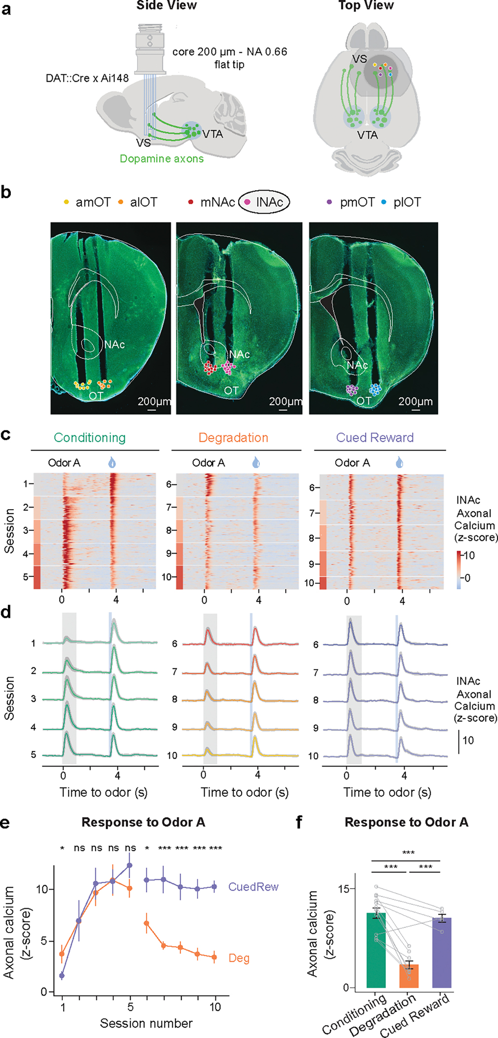
Given the well-documented role of dopamine in associative learning, we sought to characterize the activity of dopamine neurons in our task. We monitored axonal calcium signals of dopamine neurons using a multi-fiber fluorometry system with optical fibers targeting 6 locations within the ventral striatum (VS), including the nucleus accumbens (NAc, medial and lateral) and the olfactory tubercle (OT, 4 locations; Fig. 2a, b). Recordings were made only in the Deg and CuedRew groups, with the final session of Phase 1 used as the within-animal conditioning control.

Figure 2.

Dopamine axonal activity recordings show different responses to rewarding cues in Degradation and Cued Reward conditions.

(a) Configuration of multifiber photometry recordings.

(b) Coronal section from one DAT::cre x Ai148 mouse showing multiple VS fiber tracts. Only lNAc data presented in main results. lNAc, Lateral nucleus accumbens; mNAc, Medial NAc; alOT, anterior lateral olfactory tubercle; plOT, posterior lateral OT; amOT, anterior medial OT; pmOT, posterior medial OT. Points overlayed show the aligned placement for all animals (n=13).

(c) Heatmap from two mice (mouse 1, left two panels, mouse 2, right panel) illustrating the z-scored dopamine axonal signals in Odor A rewarded trials (rows), aligned to the onset of Odor A for three conditions.

(d) Population average z-scored dopamine axonal signals in response to Odor A and water delivery. Shaded areas represent SEM.

(e) Mean peak dopamine axonal signal of Odor A response by sessions for the Deg group (orange, n=8) and the CuedRew group (purple, n=5; two-sided mixed-effects model).

(f) Mean peak dopamine axonal signal for the last session in Phase 1 (Conditioning) and 2 (Degradation and Cued Reward) for both Deg (n=8) and CuedRew (n=5) groups. In panels E and F: error bars represent SEM. ns, P >0.05; *, P<0.05 ***, P < 0.001 in two-sided mixed-effects model with Tukey HSD posthoc.

To ensure similar sensor expression across the recording locations, we crossed DAT-Cre transgenic mice with Ai148 mice to express GCaMP6f in DAT-expressing neurons. Fiber locations were verified during post-mortem histology (Fig. 2b). All main text results are from the lateral nucleus accumbens (lNAc), where TD error-like dopamine signals have been observed most consistently²⁵, though the main findings are consistent across all locations (minimum cosine similarity vs. lNAc’s DA signals during Odor A rewarded trials: 0.92, Extended Data Fig. 2).

During Phase 1 (initial conditioning) dopamine axons first responded strongly to water and weakly to Odor A (Fig. 2c, d; Extended Data Fig. 3a–c). As learning progressed, the response to water gradually decreased (t₁₃ = −9.351, p < 0.001, mixed-effects model first vs. last session, Phase 1; Extended Data Fig. 3 d–f), while the response to Odor A increased over the course of 5 sessions (t₁₃ = 40.63, P < 0.001, mixed-effects model first vs. last session, Phase 1), broadly consistent with previous reports of odor-conditioning on stochastic rewards²⁰.

During contingency degradation (Deg, Phase 2), the Odor A response decreased across sessions (t₈ = −13.89, P < 0.001, mixed-effects model, session 6 vs. 10) consistent with the observed changes in anticipatory licking and recent reports of dopamine during similar tasks^7,22,23 (Fig. 2e, f). However, in the Cued Reward condition (CuedRew, Phase 2), there was a smaller decrease in the response versus the Phase 1 response (t₅ = −6.54, P < 0.001, mixed-effects model, last session Phase 1 vs. last session Phase 2), generally aligning with the behavioral results but conflicting with the idea that dopamine neurons encode contingency, at least so far as defined by $\mathrm{\Delta }P$.

In the additional phases (3–5) in the Deg group, dopamine also mirrored behavior: the Odor A response quickly recovered in Recovery 1/Phase 3, decreased during Extinction and recovered again during Recovery 2 (Phase 5; Extended Data Fig. 3c). Thus, dopamine cue responses track stimulus-outcome contingency in our Pavlovian contingency degradation and extinction paradigms though they deviated from the contingency in the CuedRew group.

TD learning models can explain dopamine responses in contingency degradation

The behavior and dopamine responses were closely aligned but not fully explained by contingency. We next tested whether TD models, successful in accounting for dopamine in other contexts, could explain our data.

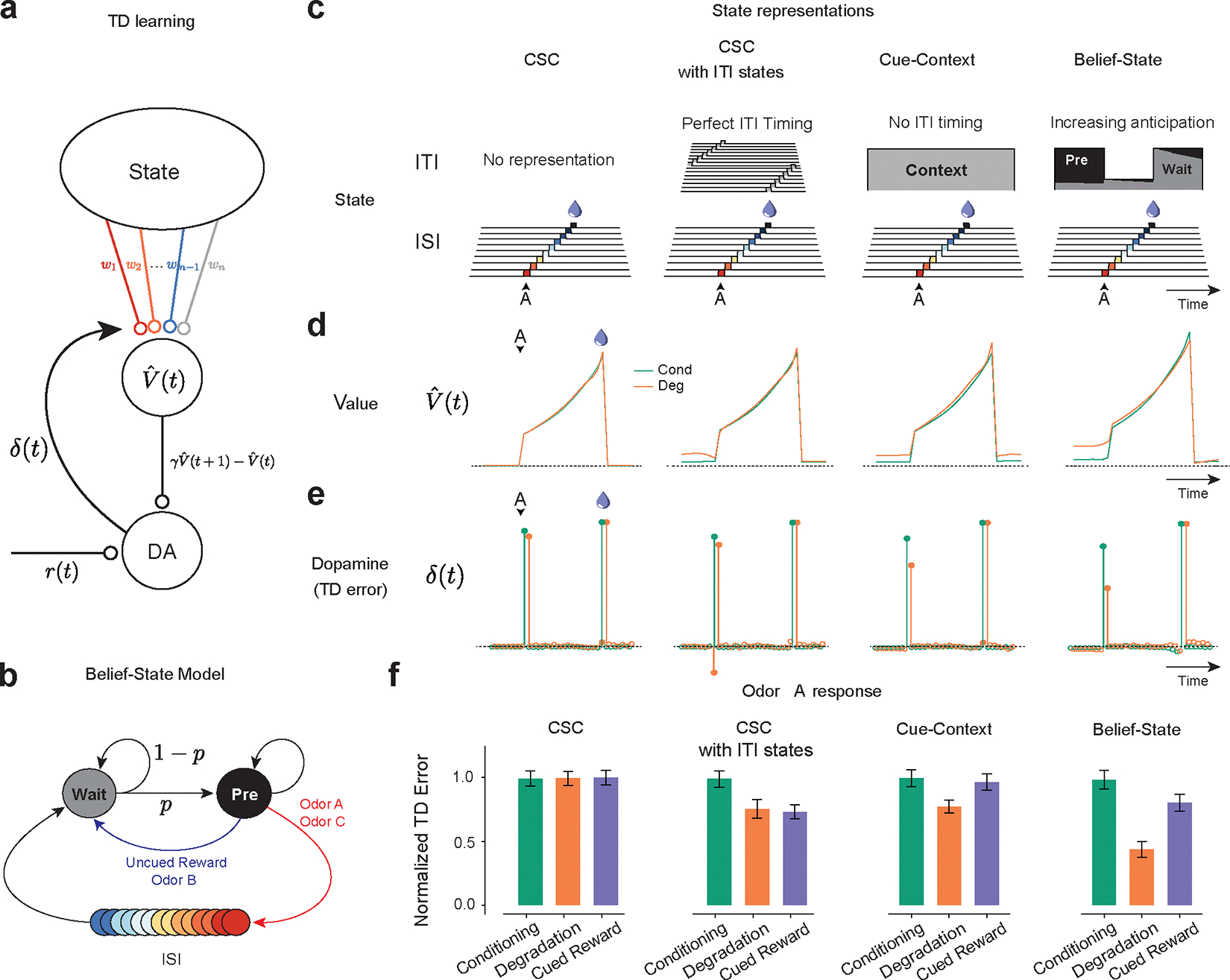
In TD models, dopamine neurons convey TD errors ($\delta )$, calculated as ${\delta }_t=r_t+\gamma V\left(s_{t+1}\right)-V\left(s_t\right)$, with $r_t$ representing reward at time $t,s_t$ being the current state, $V\left(s_t\right)$ is the value ($\mathbb{E}(\sum _{i=t}^{\infty }{\gamma }^i{r}_i)$) of state $s_t$, and $\gamma$ is the temporal discount factor. Over learning, TD errors iteratively refine the value estimate (Fig. 3a).

Figure 3.

TD learning models can explain dopamine responses in contingency degradation with appropriate ITI representation.

(a) ¬Temporal Difference Zero, TD(0), model – The state representation determines value. The difference in value between the current and gamma-discounted future state plus the reward determines the reward prediction error or dopamine. This error drives updates in the weights.

(b) Belief-State Model: After the ISI, the animal is in the Wait state, transitioning to the pre-transition (‘Pre’) state with fixed probability p. Animal only leaves Pre state following the observation of odor or reward.

(c) State representations: from the left, Complete Serial Compound (CSC) with no ITI representation, CSC with ITI states, Cue-Context model and the Belief-State model.

(d) Value in Odor A trials of each state representation using TD(0) for Conditioning and Degradation conditions

(e) TD error is the difference in value plus the reward.

(f) Mean normalized TD error of Odor A response from 25 simulated experiments. Error bars are SD.

Modeling initially focused on the response to Odor A, as this differed most between our three test conditions (Cond, Deg, CuedRew). In TD models, the Odor A response is $r_t+\gamma V\left(s_{t+1}\right)-V\left(s_t\right)=\gamma V\left(s_{t+1}\right)-V\left(s_t\right)$, the value difference between the beginning of the inter-stimulus interval (ISI) and the end of the inter-trial-interval (ITI). The assumptions of state representation affects the prediction of TD models^26–29 and thus we tested TD models (Fig. 3a) with a hand-crafted state space (Fig. 3b) and three different forms of commonly used state representation (Fig. 3c).

Many dopamine responses can be explained by simplistic state representations, with the first accounts of dopamine as a TD error using a complete serial compound state (CSC) representation^18,30. In CSC, stimuli trigger sequential activation of sub-states, only one active at a time, each representing a time step after the stimulus terminating at the outcome (Fig. 3c). This is insufficient to explain our results. The Odor A ISI is identical in all conditions and thus ISI-only CSC predicts identical results (Fig 3 d, e, f). This CSC implementation does not represent states in the ITI ($\therefore V\left(ITI\right)=0$) therefore failing, akin to the early contiguity models.

Contingency-based models are fundamentally contrastive, explaining the decrease in response by unchanged P(R|A+) and P(R|A-) increasing. Likewise, it is necessary to have state representation during the ITI for TD to explain contingency degradation. All models with ITI representation we tested explained the decrease in the Odor A response by increased in ITI value (Fig. 3d) but differed in how they modeled the changing expectation of reward during the ITI.

We explored three different state representations of the ITI, each predicting decreased Odor A response in Degradation versus Conditioning. The first (“CSC with ITI states”), extends the CSC model discussed above such that the ITI is completely tiled by substates, rather than terminating at outcome. This implicitly assumes that the animal can perfectly time out the entire task: the current substate being solely determined by time from the last trial. This model predicts a decrease for both the Degradation and Cued Reward conditions (Fig 3f.), a consequence of its perfect timing: with identical reward amount and delivery between these conditions, at any time in the ITI, the time to the next reward is the same, though there is an effect of discounting factor (Extended Data Fig. 4).

The next considered model, the “Cue-Context” model, functions similar to the previously described cue-competition model^12–15. This model has a single additional persistent state that represents context, implying there is no effect of time during the ITI on value prediction. This model successfully predicts the pattern of experimental results we observed, with a decrease in the Odor A response during Degradation and a smaller decrease during Cued Reward (Fig. 3f), with the effect size dependent on the discounting parameter (Extended Data Fig. 4 a, b). Notably, to quantitatively match our experimental results, the Cue-context model requires a discount parameter below reported values^31,32, at which cue responses are predicted to be an order of magnitude smaller than unpredicted reward responses.

Neither extreme of ITI timing well matches the experimental data. Mice probably can time the ITI, albeit with some uncertainty. Modeling temporal uncertainty can explain some discrepancies between experimental results and TD model predictions. In microstimuli models³³, cues trigger series of overlapping sub-states that decrease in intensity but increase in width, representing increasing temporal uncertainty. They were developed, in part, to explain the lack of a sharp omission response. We explored microstimuli to model our data, but there was no parameter combination that could simultaneously explain a decrease in the predicted reward response with training and the pattern of Odor A responses (Extended Data Fig. 5).

Uncertainty arises not just because of timing ability, but by the structure of the task. Mice may be able to time the approximate mean length of the ITI and use this to guide their value predictions. Inspired by previous work showing that dopamine neurons are sensitive to hidden state inference in a task with stochastically timed rewards^34,35, we next considered a ‘belief-state’ representation. In this model, value is the weighted sum of value of all possible states, weighing by the ‘belief’ (probability) of being in that state.

Unlike previous investigation³⁴, we focused on uncertainty during the ITI rather than the ISI. We did this by representing the ITI as beliefs over two possible states (Fig. 3b): a ‘Wait’ state, reflecting early ITI, and a ‘pre-transition’ (Pre) state, reflecting late ITI. For simplicity, we assumed there was a fixed rate of transition between these states (absent any observation). This means that Pre-state belief monotonically increases during the ITI following a geometric series, capturing a growing anticipation of the next trial. This model improved the quantitative accuracy of the model for a given γ versus the Cue-Context, getting sensible results using previously reported $\mathrm{\gamma }$ values (Fig 3f., Extended Data Fig. 4).

We understand the success of the Belief-State model by considering the state immediately before Odor A. At that time, the predominant belief is Pre-state. In the Degradation condition, the Pre-state value is the weighted mean of an immediate unexpected reward and a delayed, and thus discounted, cued reward. In the Cued Reward setting, both outcomes (odor A or C) are temporally discounted. Hence, Pre-state value depends on the discounting factor and transition structure (Extended Data Fig. 4). Consequently, if the interval between the reward and odor C was reduced, the model predicts there would be a greater decrease in the odor A response.

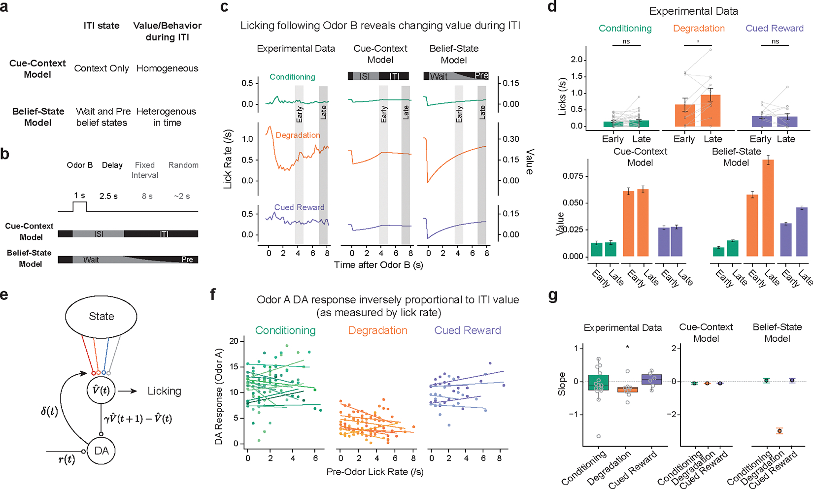
Additional behavioral and dopamine data support the Belief-State model (Fig 4a). In the Degradation condition, Odor B delivery prompted animals to stop licking, slowly beginning to lick again after several seconds. This pattern supports the Belief-State model. In Pavlovian settings, anticipatory licking (cf. consummatory licking) is often used to measure current value – with animals licking more to cues predicting greater rewards¹⁹. Odor B predicts no reward and informs that the next reward is at least one trial’s duration away. While the Cue-Context and Belief-State models can capture this decrease, the crucial difference is how the lick rate recovers. In the Cue-Context model, ITI value is related to a single state, which, without reward, decreases at the rate of $\alpha$ (learning rate). In the Belief-State model, value continually increases (Fig. 4b, c) across the entire ITI, as the increased belief that the next trial is imminent increases. The licking matches the pattern of value in the Belief-State model and not the Cue-Context model (Fig. 4c, summarized in Fig. 4d).

Figure 4.

Belief-State model, but not Cue-Context model, explains variance in behavior and dopamine responses.

(a) Cue-Context model and Belief-State model differ in their representation of the ITI.

(b) Odor B predicts no reward and at least 10 s before the start of the next trial. An ideal agent waits this out, only licking late in the ITI.

(c) Odor B induces a reduction in licking, particularly in the Degradation condition, which matches the pattern of value in the Belief-State model better than the Cue-Context model.

(d) Quantified licks (top) from experimental data in early (3.5–5s) and late (7–8s) post cue period. Error bars are SEM, *, P < 0.05, two-sided paired t-test (Conditioning, p = 0.457, n = 30; Degradation: p = 0.0413; n=11; CuedReward: p = 0.92, n = 13). Value from Cue-Context and Belief-State model for the same time period, error bars are SD.

(e) If licking is taken as a readout of value, then ITI licking should be inversely correlated with dopamine.

(f) Per animal linear regression of Odor A dopamine response (z-score axonal calcium) on lick rate in 2s before cue delivery in last two sessions of each condition.

(g) Summarized slope coefficients from experimental data (left) and models (right). Boxplot shows median and IQR; whisker are 1.5× IQR, one sample two-sided t-test (Conditioning, p = 0.27, n= 13; Degradation: p=0.057, n= 8; Cued Reward: p = 0.070, n = 5)

The Belief-State model can also explain some of the trial-by-trial variance of the dopamine response. The Belief-State model predicts an inverse correlation between pre-odor lick rate (as a measure of current value) and Odor A dopamine response. We linearly regressed the trial-by-trial pre-odor lick rate to the Odor A for each mouse finding only in the Degradation condition was there significant negative correlation (Fig. 4f, g). In Belief-State model, but not the Cue-Context model, the ITI value varies with ITI length (Fig. 4g). The lack of a significant trend in the remaining two conditions is likely due to the lower variance in value, and thus the expected effect size.

In summary, ITI representation is essential for distinguishing the effects of Degradation and Cued Reward on the Odor A response. Using many substates is ineffective, whereas using a single ITI state miss changes occurring in the ITI. Our Belief-State model is sufficient, explaining the results by using task-informed transitions between two ITI states.

Additional aspects of dopamine responses and model predictions

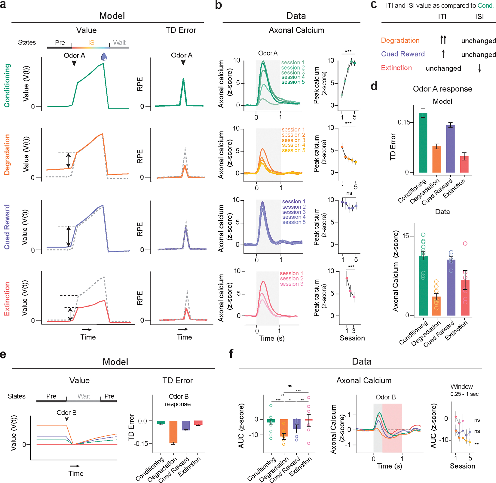
Having identified a sufficient model to the odor A results, we next examined how well this model matched all our experimental results (Figure 5). In the Odor A rewarded trial, the ISI value remained unchanged in the first three conditions, and significantly decreased in Extinction (Figure 5a), closely mirroring the prospective reward probability. For the reasons discussed above, the pre-ISI period, reflecting the pre-transition state (‘Pre’), showed a modest increase in the Cued Reward case and a significant rise in the Degradation condition. The TD errors upon Odor A presentation, reflective of the difference in value between these two substates, diminished in both Degradation and Extinction. The contingency-account explains this decrease by an increased $P\left(R\right|A-)$ and decreased $P\left(R\right|A)$, respectively³⁶. Likewise, our model suggested two mechanisms: an increase in Pre-state value in Degradation and a decrease in ISI value in Extinction (Fig. 5c). Our Belief-State TD learning model matched the experimental results well (Fig. 5b, d), including the Extinction data.

Figure 5.

Belief-State model’s predictions recapitulate additional experimental data. For all experimental summary data, n = 13 (conditioning), n = 8 (degradation), n = 5 (cued reward) and n = 7 (extinction). Error bars are SEM. ns, P >0.05; * P < 0.05, **, P < 0.01, *** P < 0.001. For all model summary n = 25 (all conditions) and error bars are SD.

(a) Plots averaged from one representative simulation of Odor A rewarded trial (n = 4,000 simulated trials) for four distinct conditions using the Belief-State model. Graphs are for the corresponding value function (left) and TD error (right) of cue response for Odor A rewarded trials.

(b) Signals from dopamine axons (mean) across multiple sessions of each condition (left). Mean peak dopamine axonal calcium signal (z-scored) for the first to last session in Phase 2 for four contingency conditions (right). Two-sided mixed-effects model. P = 0.137 for Cued Reward, P < 0.001 all other comparisons. The Belief-State model captures the modulation of Odor A dopamine response in all conditions.

(c) Degradation, Cued Reward and Extinction conditions differ in how their ITI and ISI values change compared to Conditioning phase.

(d) Mean peak TD error by Belief-State model and dopamine axonal signal (z-scored) to Odor A for four distinct conditions. The model’s prediction captured well the pattern in the dopamine data. All pairwise difference at P<0.001 are significant using two-sided mixed-effects model with Tukey’s HSD post-hoc test.

(e) Averaged traces from a representative simulation of Odor B trial (n = 4000 simulated trials) across four distinct conditions using the Belief-State model. Graphs are for the value function and TD errors of cue response for Odor B trials.

(f) Z-scored dopamine axonal signals to Odor B quantified from the red shaded area to quantify the later response only. Bar graph (left) shows mean z-scored Odor B AUC from 0.25s-1s response from the last session of each condition. Two-sided mixed-effects model with Tukey HSD post hoc. (Cond vs Cued Rew: P = 0.007; Cond vs Ext: P = 0.43; Deg vs CuedRew: P = 0.035; CuedRew vs Ext: P = 0.0051, all other P<0.001). Line graph (right) shows mean z-scored AUC over multiple sessions for each condition. Two-sided mixed-effects model, first and last sessions of these conditions (Degradation: P<0.001; CuedRew P = 0.62; Extinction P = 0.74).

The Belief-State model accurately predicts differences in the odor B response between conditions. In Degradation, TD error for all cues changes as the shared Pre-state value changes, while Extinction impacts only the cue undergoing extinction. In our model, Odor B is a transition from the Pre to Wait state, and thus the TD error is the difference between these two state values. We expected the most negative response in the Deg group, owing to a higher Pre state value, and relatively unchanged ‘Wait’ value and we expected an unchanged response in Extinction in comparison to Conditioning. Experimentally, the response to Odor B was biphasic, featuring an initial positive response followed by a later negative response. Such a biphasic response has been previously noted in electrophysiological data, with general agreement that the second phase is correlated with value³⁷. Quantifying the later response (250ms-1s), there was a close match between the model prediction and the data for Odor B responses (Fig. 5e, f).

The Belief-State model shows that TD errors at reward omission are based on the difference between the final ISI substate and Wait state values. The Wait state value, generally lower than the Pre state value, is relatively unchanged between conditions. This results in consistent TD errors at reward omission across Conditioning, Degradation, and Cued Reward conditions due to similar ISI values, but a significant reduction in Extinction due to a lower ISI value, closely aligning with the experimental data (Extended Data Fig. 6). Similarly, predicted reward responses was relatively unchanged; in TD these responses are the difference between actual reward and ISI values, which are unchanged between conditions in the modeling and exhibit minimal changes in our data (Extended Data Fig. 6f). In total, the TD model with proper task states effectively recapitulates nearly all aspects of phasic dopamine responses in our data.

Recurrent neural networks that learn to predict values through TD learning can explain dopamine responses

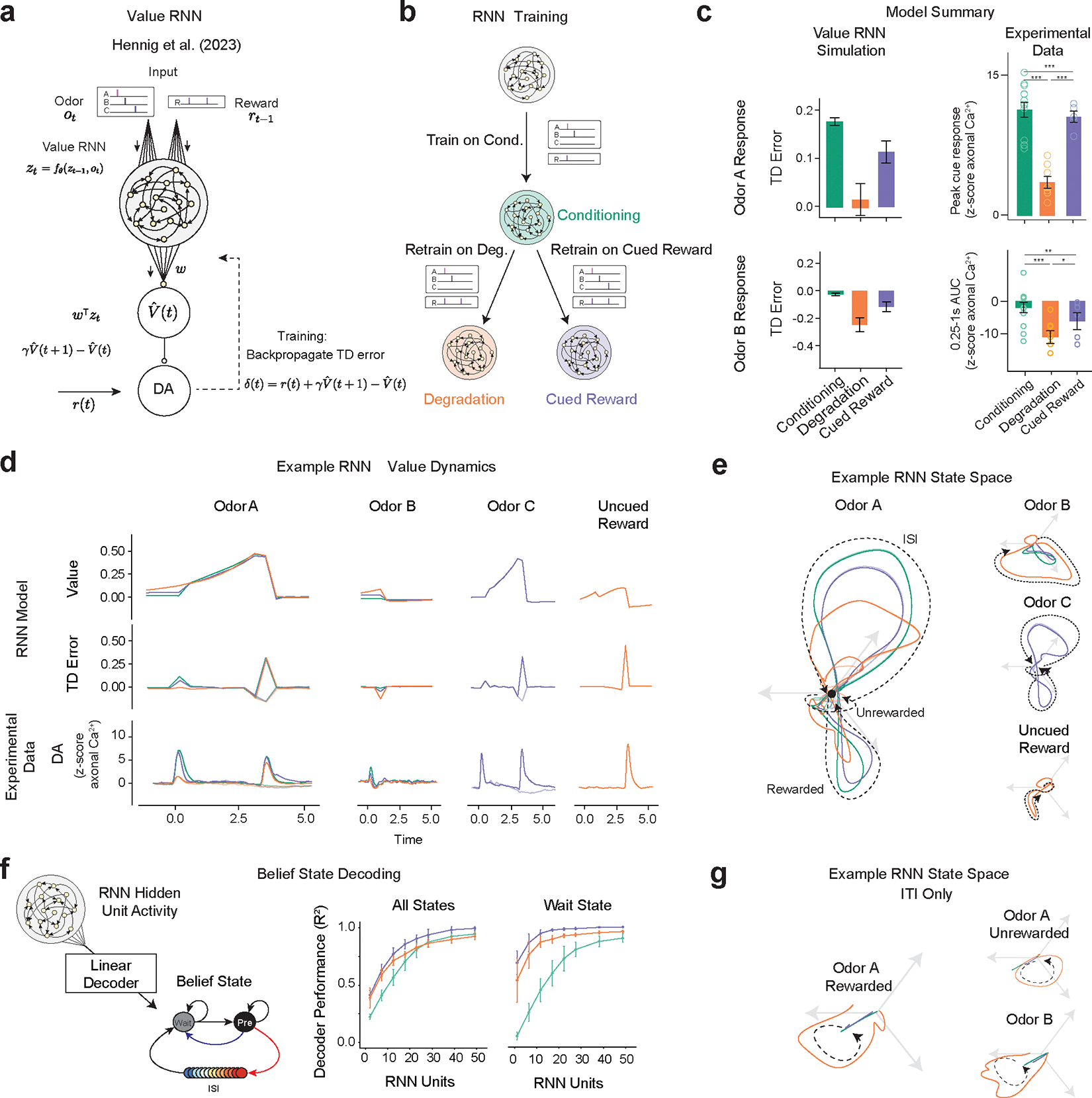
Our work above adds another task to the several already documented^34,35,38, where dopaminergic activity can be explained by belief-state TD models. But these models are ‘hand-crafted,’ tuned for the particular task setting. How the brain learns such state-spaces is poorly understood. Previous work showed RNNs, trained to estimate value directly from observations (‘value-RNNs’), without aiming to, develop belief-like representations³⁹. This approach substitutes hand-crafted states for an RNN that is only given the same odor and reward observations as the animal (Fig. 6a).

Figure 6.

Value-RNNs recapitulate experimental results using state-spaces akin to hand-crafted Belief-State model. For all panels, experimental data: Conditioning (n=13), Degradation (n = 8), Cued Reward (n = 5) error bars are SEM, Extinction (n=7); models (n=25 simulations) error bars are SD;

(a) The Value-RNN replaces the hand-crafted state space representation with an RNN that is trained only on the observations of cues and rewards. The TD error is used to train the network.

(b) RNNs were initially trained on simulated Conditioning experiments, before being retrained on either Degradation or Cued Reward conditions.

(c) The asymptotic predictions of the RNN models (mean, error bars: SD, n = 25 simulations, 50-unit RNNs) closely match the experimental results (see Figure 2f, 5f for statistics). * P < 0.05, **, P < 0.01, *** P < 0.001

(d) Example value, TD error, and corresponding average experimental data from a single RNN simulation. Notably, decreased Odor A response is explained by increased value in the pre-cue period.

(e) Hidden neuron activity projected into 3D space using CCA from the same RNNs used in (d). The Odor A ISI representation is similar in each of the three conditions, and similar to the Odor C representation. Odor B representation is significantly changed in the Degradation condition.

(f) Correspondence between RNN state space and Belief-State model. A linear decoder was trained to predict beliefs using RNN hidden unit activity. With increasing hidden layer size (n=25 each layer size), the RNN becomes increasingly belief-like. The improved performance of the decoder for the Degradation condition is explained by better decoding of the Wait state. Better Wait state decoding is explained by altered ITI representation.

(g) Same RNNs as in (d) and (e), hidden unit activity projected into state-space as (e) for the ITI period only reveals ITI representation is significantly different in the Degradation case.

Here, we applied the same value-RNN to our contingency manipulation experiments. The RNNs (≤50 hidden units) were first trained in Conditioning and then on Degradation or Cued Reward conditions (Fig. 6b). The trained RNNs closely matched the experimental data (example 50-unit RNN in Fig. 6c). Like the TD models used in the above section, the decrease in Odor A response is explained by an increase in the value during the ITI period (example Fig. 6d).

We next investigated the state spaces used by the RNN models, applying canonical correlation analysis (CCA, Extended Data Fig. 7) to align the hidden unit activity. In all conditions, without any stimuli, the RNNs’ activity decayed to a fixed point (Supplementary Video 1) that can be understood as the Pre-transition state. In all conditions, the Odor A trajectory is similar, reflecting a shared representation of the ISI period (Fig. 6e). Moreover, in the Cued Reward condition, the Odor C trajectory is nearly identical to Odor A, suggesting generalization. Odor B trajectories were significantly longer in the Degradation condition, potentially reflecting the Wait state.

To compare the state space of the value-RNN to the Belief-State model, we regressed simulated beliefs onto hidden unit activity. As previously noted³⁹, unit activity became more belief-like with more hidden units (Fig. 6f). As evident in the visualized state spaces, the RNNs trained on the Degradation condition developed distinct trajectories in the ITI compared to the other two conditions (Fig. 6g), taking longer to return to the fixed ITI point. The return trajectory was similar regardless of the trial type. In all RNNs that successfully predicted degradation reduced odor A response, the Wait-state readout had a minimum performance of $R^2=0.57$, suggesting the delivery of rewards during the ITI that reshapes the state space to be heterogeneous. In other conditions the ITI has a relatively fixed state space representation. We take the RNN can learn a belief-like representation from limited information, using only the TD error as feedback, to suggest a generalized method by which the brain can construct state spaces using TD algorithms.

A retrospective learning model, ANCCR, cannot explain the dopamine responses

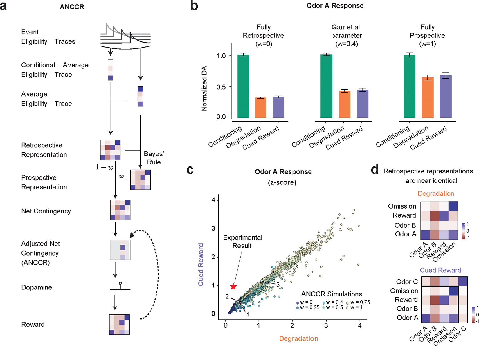
While the success of both our Belief-State TD model the value-RNNs suggest that TD is sufficient to explain our results, we also investigated if alternative definitions of contingency accounted for our results. The recently-proposed ANCCR (adjusted net contingency for causal relations) is an alternative account of the TD explanation of dopamine activity (Fig. 7a)²². The authors have previously shown that this model can account for contingency degradation^22,23 and suggested that TD accounts could not.

Figure 7.

ANCCR does not explain the experimental results:

(a) Simplified representation of ANCCR model. Notably the first step is to estimate retrospective contingency using eligibility traces.

(b) Simulations of the same virtual experiments (n = 25) used in Figure 3 using ANCCR, using the parameters in Garr et al., 2024 varying the prospective-retrospective weighting parameter (w). Error bars are SD. In all cases the predicted Odor A response is similar in the Degradation and Cued Reward conditions.

(c) No parameter combination explains the experimental result. Searching 21,000 parameter combinations across six parameters (T ratio = 0.2–2, α = 0.01–0.3, k = 0.01–1 or 1/(mean inter-reward interval), w =0–1, threshold = 0.1–0.7, αR = 0.1–0.3). Experimental result plotted as a star. Previously used parameters (Garr et al., 2024 as 1, Jeong et al., 2022 as 2 and 3) indicated. Dots are colored by the prospective-retrospective weighting parameter (w), which has a strong effect on the magnitude of Phase 2 response relative to Phase 1.

(d) As the contingency is calculated as the first step, and the contingencies are similar in Degradation and Cued Reward conditions, there is little difference in the retrospective contingency representation between the two conditions, explaining why regardless of parameter choice ANCCR predicts similar responses.

ANCCR builds upon the authors’ previous observation that the retrospective information (‘which cues precede reward?’) can explain animal behavior previously unexplained by prospective accounts⁴⁰. The first step in ANCCR is the calculation of the retrospective contingency, using eligibility traces to compute contingency, generalizing the trial-based definition of $\mathrm{\Delta }{P}_{retro}\left(A\right)$ to continuous time. This is done by subtracting average cue eligibility from eligibility conditioned on an event. From this prospective contingency is recovered using a Bayes-like computation. Using both prospective and retrospective contingencies, a weighted-sum (‘net’) contingency is calculated for all event pairs. This can then be used to calculate the change in expectation of reward for a given event, considering other explanations. It is this ‘adjusted net contingency’ that is proposed to be represented in the dopamine signal.

To test the ANCCR model, we used the authors’ published code to model the same simulated experiments used in our TD modeling. We first tried using the parameters published in Garr et al. (2024) and Jeong et al. (2022); presenting results using the former as they are closer to our results. While the ANCCR model accurately predicted a decreased response for Odor A during contingency degradation, it predicted a similar response in the Cued Reward condition, conflicting with the experimental results (Fig. 7b). We varied the relative amount (w) of retrospective and prospective information used in the computation. This affected the magnitude of the decrease but not the ratio between the Cued Reward and Degradation conditions. We investigated if this was a problem of parameter selection, as ANCCR has 12 parameters, and therefore simulated the experiments for the parameter search space specified in Garr et al. (2024), ultimately trying a total of 21,000 combinations, including those in the two previous studies^22,23 (indicated as 1, 2 and 3). Fig. 7c plots the Odor A dopamine response in the Degradation and Cued Reward case for each of these combinations, normalized by the response during Conditioning. No parameter combination predicted the correct pattern of experimental results, quantitatively or qualitatively (Fig. 7c).

Discussion

We examined behaviors and VS dopamine signals in a Pavlovian contingency degradation paradigm, including a pivotal control. Our results show that dopamine cue responses, like behavioral conditioned responses, were attenuated when stimulus-outcome contingency was degraded by the uncued delivery of additional rewards. Crucially, conditioned responses were not affected, and the dopamine response was significantly less reduced, in a control condition in which additional rewards were cued by a different stimulus despite similar number of rewards. Contrary to previous claims^22,23, we could explain many aspects of dopamine responses with TD models equipped with proper state representations that reflected uncertainty inherent in the task structure. These models readily explained dopamine cue responses in the control condition with cued additional rewards – results which strongly violated the predictions of the ΔP definition of contingency and a contingency-based retrospective model (ANCCR). The results indicate that dopamine signals and conditioned responding primarily reflect the prospective stimulus-outcome relations. Rather than discarding the notion of contingency altogether, we propose that these results point toward a novel definition of contingency grounded in the prospective-based TD learning framework.

TD learning model as a model of associative learning

Pavlovian contingency degradation paradigms were pivotal in the historical development of animal learning theories^1,12. We show that the effect of contingency manipulations, both on behavior and dopamine responses, can be explained by TD learning models. The failure of previous efforts to explain contingency degradation with TD learning models is due to the use of inappropriate state representations, particularly of the ITI. We show two types of TD learning models that explain the basic behavioral and dopamine results: the Cue-Context model) and the Belief-State model.

In both models, the reduction in dopamine cue responses occurs due to an increase in the value preceding a cue presentation, which decreases the cue-induced change in value. It may be that this, in turn, explains the reduction of cue-induced anticipatory licking during contingency degradation, if this behavior is driven at least in part by the dopamine RPE^41,42.

Our results favor the Belief-State model over the Cue-Context model, both dopamine and behavioral data being better explained by the Belief-State model. Moreover, we show that RNNs, trained to predict value (value-RNNs), acquired activity patterns that can be seen as representing beliefs, merely from observations, similar to our previous work using different tasks³⁹. Critically, when trained on contingency degradation sessions, value-RNNs developed more heterogeneous representations of the ITI, the key feature to the success of our Belief-State model.

This success of the Belief-State model results from the state representation capturing the inherent uncertainty of the task structure (‘state uncertainty’), particularly the random length of the ITI. The microstimuli model³³ addresses a different kind of uncertainty, internal temporal uncertainty, and incorporating only this internal temporal uncertainty was insufficient to explain our results (Extended Data Fig. 5). Some models, (e.g.³⁰), incorporate both these uncertainties and may be expected to more fully explain all dopamine features, albeit with a greater number of parameters.

State representations as population activity dynamics

In reinforcement learning (RL), “state” is a critical component representing the observable and inferred variables necessary to compute value and policy. Critiques have highlighted the artifice of the representations used in neurobiological RL modeling, such as the implausibility of having sequentially activated neurons completely tiling the ITI, as in the CSC with ITI states model⁴³. Moreover, states are often defined within the artifice of a “trial”⁴³. What does a realistic state representation look like? The success of value-RNNs in replicating our experimental data provides two crucial insights into how biological circuits may represent states.

First, the dynamics of artificial neural networks provides a useful construction of state space. Our success with our relatively small value-RNNs echoes the recent successes of RL on complex tasks with many stimuli and without obvious trial structure, which demonstrated high performance is possible with standard RL techniques¹⁷, with the key being neural networks that autonomously learn task-appropriate representations. In our previous work³⁹ and this work, value-RNNs have a stable fixed point (attractor) corresponding to the ITI state (Pre-transition state of our Belief-State model) as an emergent property of training to predict value whereas the stimulus-specific trajectories closely corresponded to the hand-crafted states assumed in Belief-State TD learning models. The population activity patterns of network, including attractors and stimulus-specific trajectories act as appropriate state representations. While this likely involves overlapping sets of neurons, value can still be learnt using TD to adjust the readout synaptic weights.

Second, while hand-crafted state representations can advance conceptual understanding, the RNN-based approach provides insights into biological implementation. In future, the activity of value-RNNs may be a useful framework to study neural activity in the brain thought to encode state. For example, it is already known the prefrontal cortex receives VTA-dopaminergic innervation that is necessary for appropriate adaptation to contingency degradation during instrumental conditioning⁴⁴. Value-RNNs suggest a mechanism of this adaptation. We do note other areas, such as the hippocampus, also contribute task-relevant information during degradation to the prefrontal cortex⁴⁵. Moreover, modeling approaches reflecting the brain’s functional organization (e.g. ⁴⁶) might provide more insight than considering the brain’s state-machinery as a single RNN.

Limitations of the ANCCR model as a model of associative learning and dopamine

The present study unveiled limitations of the recently proposed causal learning model, ANCCR^22,23. Our Degradation and Cued Reward conditions are minimally different and provide a strong test of ANCCR’s algorithm design. ANCCR fails to explain the observed results despite our extensive exploration of its parameter space. While contending with both continuous time and multiple cues, ANCCR suffers the same flaw as the $\Delta P$ definition of contingency: contingency is computed by subtracting the average event rate, losing the evolving, state-conditional information during the ITI that was necessary for the TD models to work. The similar event rates between our conditions means the retrospective representations average eligibility trace and thus retrospective contingency are also similar (Fig 7d). Thus, ANCCR predictions are similar for the two conditions, not because of parameter choice, but because of the fundamental construction of the model, as retrospective contingency is the input to the entire model.

The failure of the ANCCR model here does not exclude some of the interesting ideas integrated into ANCCR, including using retrospective information to learn state space. Further, it also assumes that certain parameters, specifically eligibility trace decay parameters, are a function of task parameters, giving it the timescale invariance properties noted by Gallistel that is not a feature of TD models with fixed learning parameters⁴⁷. Such flexibility may improve the accuracy of TD simulations using simpler models (e.g. Cue-Context).

A recent report²³ demonstrated that ANCCR is able to explain the dopamine response in outcome-selective contingency degradation. This is a result of the multidimensional tracking of cue-outcome contingencies in ANCCR. We show that both the Belief-State model and the value-RNN can successfully predict these experimental results (Extended Data Fig. 8), similar to how “multi-threaded predictive models” have explained dopamine data in a different multi-outcome task²⁹. The recent studies evidencing heterogeneous dopamine responses to different rewards types^48,49 may be a more useful avenue to understanding the biology and thus constraining the models of multi-outcome learning.

TD error, contingency and causal inference

Learning predictive and causal relationships requires assigning credit for the outcomes to correct events and key to this is considering counterfactuals⁵⁰ – would an outcome occur had I not seen that cue? Here, the subtraction of value immediately before cue presentation is core to explaining the dopamine responses. This can be seen as subtracting the prediction made in the absence of the cue, i.e. the counterfactual prediction. More generally, the computation of TD error or its variants can be considered to subtract out counterfactuals; in advantage actor-critic algorithms (a RL algorithm class used frequently in machine learning), the benefit of an action is evaluated using the advantage function:

$$A\left(s_t,a_t\right)=Q\left(s_t,a_t\right)-V\left(s_t\right)$$

where ${Q(s}_t,a_t)$ is the state-action value function^51,52. If ${Q(s}_t,a_t)$ is the immediate reward of the action plus the expected return of the new state, $Q\left(s_t,a_t\right)=r_t+\gamma V\left(s_{t+1}\right),$ then the advantage function can be approximated by the TD error $A\left(s_t,a_t\right)=Q\left(s_t,a_t\right)-V\left(s_t\right)=\left(r_t+\gamma V\left(s_{t+1}\right)\right)-V\left(s_t\right)={E[\delta }_t]$ (^53,54). In fully-observable environments without confounds, the advantage function is the Neyman-Rubin definition of causal effect of an action⁵⁴: the difference in outcomes given an action versus otherwise. In this admittedly artificial context, the definitions of causality, contingency and TD error align. TD error can therefore measure contingency and guide causal learning, without invoking retrospective computations.

TD errors improve over the ANCCR and $\mathrm{\Delta }P$ definitions because the comparison is not simply to absence of CS, but to $V\left(s\right)$, the γ-discounted sum of all future rewards given the current state, encapsulating information beyond mere cue absence. As our modeling demonstrates, the state representation during eventless periods (ITI) is critical to the accuracy of our models. Here, we have not explored how state representation is learnt, comparing fully learnt responses to the TD and RNN models. Under our straightforward Pavlovian setup, our value-RNN can discover states and causality because causality is reduced to outcome prediction⁵⁵. It is more challenging in partially observable environments⁵⁰ and instrumental paradigms. While the batch learning of our value-RNN is biologically-implausible, active research in the RL literature continues to seek efficient, online methods to use counterfactual considerations to implement state and causality learning⁵⁶,⁵⁷.

Conclusions

Our results show TD learning models can explain contingency degradation – a phenomenon previously thought difficult to explain with TD learning^22,23,58. Sensitivity to contingency degradation in instrumental behaviors is often used to label behavior as goal-directed or model-based. But our model can, in principle, be applied to explain such behavior but is not neatly classified as “model-free” or “model-based”. It is model-based in using cached state-values based on direct experience, but state depends on the world model of the learnt transition structure^26,28,59. Our results are an important step to understanding the link between behavior and contingency, in doing so, stepping towards an understanding of how the brain learns causality.

Methods

Animals

A total of 31 mice were used. 18 wildtype mice (8 males and 10 females) at 3–6 months of age were used to collect only behavioral data. For fiber photometry experiments, 13 double transgenic mice resulting from the crossing of DAT-Cre (Slc6a3tm1.1(cre)Bkmn; Jackson Laboratory, 006660)⁶⁰ with Ai148D (B6.Cg-Igs7tm148.1(tetO-GCaMP6f,CAG-tTA2)Hze/J; Jackson Laboratory, 030328)⁶¹ (DAT::cre x Ai148, 7 males and 6 females) at 3–6 months of age were used. Mice were housed on a 12 hr /12 hr dark/light cycle. Ambient temperature was kept at 75 ± 5 °F and humidity below 50%. All procedures were performed in accordance with the National Institutes of Health Guide for the Care and Use of Laboratory Animals and approved by the Harvard Animal Care and Use Committee.

Surgery

Mice used for fiber photometry recordings underwent a single surgery to implant a multifiber cannula and a head fixation plate 2–3 weeks prior to the beginning of the behavioral experiment. All surgeries were performed under aseptic conditions. Briefly, mice were anesthetized with an intraperitoneal injection of a mixture of xylazine (10 mg/kg) and ketamine (80 mg/kg) and placed in a stereotaxic apparatus in a flat skull position. During surgery, the bone above the Ventral Striatum area was removed using a high-speed drill. A custom multifiber cannula (6 fibers, 200 μm core diameter, 0.37 NA, Doric Lenses) was lowered over the course of 10 min to target 6 subregions in the Ventral Striatum. The regions’ coordinates relative to Bregma (in mm) were: Lateral nucleus accumbens (lNAc, AP:1.42, ML:1.5, DV:−4.5); Medial NAc (mNAc, AP:1.42, ML:1, DV:−4.5); anterior lateral olfactory tubercle (alOT, AP:1.62, ML:1.3, DV:−4.8); posterior lateral OT (plOT, AP:1.00, ML:1.3, DV:−5.0); anterior medial OT (amOT, AP:1.62, ML:0.8, DV:−4.8); posterior medial OT (pmOT, AP:1.00, ML:0.8, DV:−5.0). Dental cement (MetaBond, Parkell) was then used to secure the implant and custom headplate and to cover the skull. Mice were singly housed after surgery and post-operative analgesia was administered for 3 days (buprenorphine ER-LAB 0.5 mg/ml). Mice used for behavioral training underwent a similar surgical process, but only a head fixation plate was implanted.

Behavioral training

After recovery from headplate-implantation surgery, animals were given ad libitum access to food and water for 1 week. Before experiments and throughout the duration of the experiments, mice were water restricted to reach 85–90% of their initial body weight and provided approximately 1–1.5 mL water per day in order to maintain the desired weight and were handled every day. Mice were habituated to head fixation and drinking from a waterspout 2–3 days prior to the first training session. All tasks were run on a custom-designed head-fixed behavior set-up, with software written in MATLAB and hardware control achieved using a BPod state machine (1027, Sanworks). A mouse lickometer (1020, Sanworks) was used to measure licking as infra-red beam breaks. The water valve (LHDA1233115H, The Lee Company) was calibrated, and a custom-made olfactometer was used for odor delivery. The odor valves (LHDA1221111H, The Lee Company) were controlled by a valve driver module (1015, Sanworks) and a valve mount manifold (LFMX0510528B, The Lee Company). All components were controlled through the Bpod state machine. Odors (1-hexanol, d-limonene, and ethyl butyrate, Sigma-Aldrich) were diluted in mineral oil (Sigma-Aldrich) 1:10, and 30 μL of each diluted odor was placed on a syringe filter (2.7-μm pore size, 6823–1327, GE Healthcare). Odorized air was further diluted with filtered air by 1:8 to produce a 1 liter/min total flow rate. The identity of the rewarded and non-rewarded odors were randomized for each animal.

In Conditioning sessions, there are three types of trials: (1) trials of Odor A (40% of all trials) associated with a 75% chance of water delivery after a fixed delay (2.5 s), (2) trials of unrewarded Odor B (20% of all trials) as control to ensure that the animals learned the task, and (3) background trials (40% of all trials) without odor presentation. Rewarded Odor A trials consist of 2s pre-cue period, 1s Odor A presentation, 2.5s fixed delay prior to a 9 μL water reward and 8s post-reward period. Unrewarded Odor B trials consist of a 2s pre-cue period, 1s Odor B presentation, and 10.5s post-odor period. Background trials in the Conditioning phase span a 13.5s eventless period. Trial type was drawn pseudo-randomly from a scrambled array of trial types maintaining a constant trial type proportion. Inter-trial-intervals (ITI) following the post-reward period were drawn from an exponential distribution (mean: 2s) or a truncated exponential distribution (mean: 2.5s, truncated at 6s; fixed post-reward period reduced from 4s to 8s). We did not observe a difference between the results from the two trial timings and present them combined. No additional timing cues were given either to indicate trial timing or reward omission.

Learning was assessed principally by anticipatory licking detected at the waterspout for each trial type, with mice performing 100–160 trials per session until they reach an asymptotic task performance, typically after 5 sessions.

After the Conditioning phase, the mice were divided into three groups to undergo different conditions: Degradation (Deg group), Cued Reward (CuedRew group), and Conditioning (Cond group). The Deg group experienced contingency decrease during the Degradation phase. In the Degradation phase, Odor A still delivers water reward with 75% probability, and Odor B remains unrewarded. The difference was the introduction of uncued rewards (9 μL water) in 75% of background trials to diminish the contingency. Animals underwent 5 sessions, each with 100–160 trials, to adapt their conditioned and neural responses to the new contingency. Degradation changed the cue value relative to the background trial but did not impact the reward identity, reward magnitude, or delay to/probability of expected reward.

The CuedRew group was included to account for potential satiety effects due to the extra rewards the Deg group mice received in the background trials. Unlike the Deg group, the CuedRew group’s background trials were substituted with rewarded Odor C trials, where mice received additional rewards signaled by a distinct odor (Odor C). Rewarded Odor C trials have the same trial structure as the rewarded Odor A trials and animals were given 5 sessions, with 100–160 trials each, to adapt their conditioned response and neural responses to this manipulation.

The Cond group proceeded with an additional five Conditioning sessions, keeping the trial structure and parameters unchanged as in the Conditioning phase.

Post-degradation: eight mice were randomly chosen from the Deg group for the reinstatement phase, replicating the initial Conditioning conditions. After three reinstatement sessions, once the animals’ performance rebounded to pre-degradation levels, we initiated the extinction process. This involved the delivery of both odors A and B without rewards, effectively extinguishing the cue-reward pairing. To mitigate the likelihood of animals generating a new state to account for the sudden reward absence, a shorter reinstatement session was conducted prior to the Extinction session on the extinction day. Extinction was conducted over three days, each day featuring 100–160 trials. After Extinction, a second reinstatement session was implemented, re-introducing the 75% reward contingency for Odor A. All eight animals resumed anticipatory licking within ten trials during this reinstatement.

Fiber photometry

Fiber photometry allows for recording of the activity of genetically defined neural populations in mice by expressing a genetically encoded calcium indicator and chronically implanting optic fiber(s). The fiber photometry experiment was performed using a bundle-imaging fiber photometry setup⁶²

(BFMC6_LED(410–420)_LED(460–490)_CAM(500–550)_LED(555–570)_CAM(580–680)_FC, Doric Lenses) that collected the fluorescence from a flexible optic fiber bundle (HDP(19)_200/245/LWMJ-0.37_2.0m_FCM-HDC(19), Doric Lenses) connected to a custom multifiber cannula containing 6 fibers with 200-μm core diameter implanted during surgery. This system allowed chronic, stable, minimally disruptive access to deep brain regions by imaging the top of the patch cord fiber bundle that was attached to the implant. Interleaved delivery 473 nm excitation light and 405 nm isosbestic light (using LEDs from Doric Lenses) allows for independent collection of calcium-bound and calcium-free GCaMP fluorescence emission in two CMOS cameras. The effective acquisition rate for GCaMP and isosbestic emissions was 20Hz. The signal was recorded during each session when the animals were performing the task. Recording sites which had weak or no viral expression or signal were excluded from analysis.

The global change of signals within a session was corrected by a linear fitting of dopamine signals (473nm channel) using signals in the isosbestic channel during ITI and subtracting the fitted line from dopamine signals in the whole session. The baseline activity for each trial (F_{0 each}) was calculated by averaging activity in the pre-stimulus period between −2 to 0 seconds before an odor onset for odor trials or water onset for uncued reward trials. Z-score was calculated as (F − F_{0 each})/STD_ITI with STD_ITI the standard deviation of the signal during the ITI.

To quantify Odor A responses, we looked for ‘peak responses’ by finding the point with the maximum absolute value during the 1-s window following the stimulus onset in each trial. To quantify Odor B responses, we measured area under curve by summing the value during the 250 ms to 1s window following the stimulus onset in each trial. This is to separate out the initial activation (odor response) that we consistently observed, and which may carry salience or surprise information independent of value. To quantify reward responses, we looked for ‘peak responses’ by finding the point with the maximum absolute value during the 1.5-s window following the reward onset in each trial. The latency between reward delivery and the first lick after reward influenced the average reward response. For long latencies, there was a biphasic response, which suggests there may be sensory cues that predict reward delivery

To quantify reward omission responses, we looked for area under curve by summing the value during the following the reward omission in each trial. This was necessary because of the temporal resolution of photometry⁶³: sensor dynamics, here of intracellular calcium, is a relatively slow measure of cell activity, and the fast on-dynamics and slow off-dynamics of the fluorescent sensor and the dynamics of intracellular calcium may blur two-component responses³⁷ together.

In analyzing photometry data, we investigated the connection between the behavior and the dopamine response on a trial-by-trial basis. When there was a long delay in the time from the first lick after a predicted or unpredicted reward, there was a biphasic response (Extended Data Fig. 3) suggesting that there may be some sensory cues associated with reward delivery. To remove this potential confound, when analyzing reward responses, we only included trials in which the lick latency to reward was less than 250 ms. This corresponds to 59% of rewards delivered after Odor A in the first session, 80% in the second session and at least 86% of trials on all other sessions. We also excluded any trial in which there was no licking detected at all. These trials were usually at the end of the session when the mouse disengaged with the task.

Histology

To verify the optical fiber placement and GCaMP expression, mice were deeply anesthetized with an overdose of ketamine-medetomidine, and perfused transcardially with 0.9% saline followed by 4% paraformaldehyde (PFA) in PBS at the end of all experiments. Brains were removed from the skull and stored in PFA overnight followed by 0.9% saline for 48 hours. Coronal sections were cut using a vibratome (Leica VT1000S). Brain sections were imaged using fluorescent microscopy (AxioScan slide scanner, Zeiss) to confirm GCaMP expression and the location of fiber tips. Brain section images were matched and overlaid with the Paxinos and Franklin Mouse Brain Atlas cross-sections to identify imaging location. No data from the lNAc fibers (main results) were excluded due to fiber placement. Some of the olfactory tubercule sites had no discernible signal and were excluded from the analysis in Extended Data Fig. 2, site specific n-values are reported in that figure.

Computational Modeling

Simulated Experiments

To compare the various models, we generated 25 simulated experiments of Cond, Deg and CuedRew groups, matching trial statistics to the experimental settings, but increasing the number of trials to 4,000 in each phase to allow to test for steady-state response in both these TD simulations and the ANCCR simulations. We then calculated the state representation of the simulated experiments for each of four state representations (CSC with and without ITI states, Context-TD, Belief-State model, detailed below) and ran the TD learning algorithm with no eligibility trace, called TD(0), using these state representations (Fig. 3a). While we used only a one-step tabular TD(0) model, but multistep and continuous formulations should converge to similar results¹⁶. TD(0) has a learning rate parameter ($\alpha$), but it did not influence the steady-state results, which are presented, and thus the only parameter which influenced the result was $\gamma$, the temporal discount factor, set to 0.925 for all simulations using a timestep of Δt = 0.2s (Extended Data Fig. 4 shows the $\gamma$ parameter search space). Code for generating the simulated experiments and implementing the simulations can be found at: https://github.com/mhburrell/Qian-Burrell-2024

CSC-TD model with and without ITI states

We initially simulated the Conditioning, Degradation, and Cued Reward experimental conditions using the CSC-TD model, adapted from Schultz et al.¹⁸. The cue length was fixed at 1 unit of time, with time unit size set to 0.2 s, and the ISI was matched to experimental parameters at 3.5 s. Simulated cue and reward frequencies were matched to experimental parameters, separately simulating Conditioning then Degradation and Conditioning then Cued Reward. In complete serial compound, also known as tapped-delay line, each cue results in a cascade of discrete substates that completely tile the ISI. TD error and value were then modelled using a standard TD(0) implementation¹⁶, using $\alpha =0.1,\gamma =0.925$. Reported values are the average of the last 200 instances averaged for 25 simulations. The model was run with states tiling the ISI only (CSC) or tiling the ISI and ITI until the next cue presentation (CSC with ITI states).

Context-TD model

The Context-TD model, which is an extension of the CSC-TD model, includes context as an additional cue, but otherwise identical to the CSC simulations. For each phase (Conditioning, Degradation, Cued Reward) a separate context state was active for the entire phase, including the ISI and ITI. This corresponds to the additive Cue-Context model previously described^12,13,15. TD errors reported are the average of the last 200 instances averaged for 25 simulations.

Belief-State model

We simulated the TD error signaling in all four conditions (Conditioning, Degradation, Cued Reward, Extinction) using a previously described belief-state TD model³⁴. For comparison to the CSC based models described above, we had a total of 19 states, 17 capturing the ISI substates (3.5s in 0.2s increments, as in the CSC model). State 18 we termed the ‘Wait’ state and state 19 the ‘pre-transition’ or ‘pre’ state. In the Belief-State model it is assumed the animal has learned a state transition distribution. We computed the transition matrix by labelling the simulated experiments with state, labelling the fixed post-US period as the Wait state and the variable ITI as the Pre state and then empirically calculating the transition matrix for that simulation. While the post-US and variable ITI periods were used to estimate the rate of transition between the Wait and Pre states, because we assumed a fixed probability of transition, these should not be considered identical – rather the implicit assumption in modeling with a fixed probability is that the time in the Wait state is a geometric random variable.

The Belief-State model also assumes that the animal has learned a probability of distributions given the current state, encoded in an observation matrix. In our implementation there are five possible observations: Odor A, B, C, reward and null (no event). Like the transition matrix, the observation matrix was calculated empirically from the simulated experiments. Fig 3b represents schematically the state-space of the Belief-State model: Odor A (and C in Cued Reward) are observed when transitioning from Pre to the first ISI state; reward is observed in transition from the last ISI state to Wait, Odor B (and reward in Deg) are observed when transitioning from Pre to Wait. We did not consider the details of how the transition and observation matrices may be learnt on a trial-by-trial basis as the steady-state TD errors are not dependent on this implementation. Figure 3c shows an example of the beliefs over a single trial. At the delivery of Odor A, the belief becomes 75% that they are in a rewarded trial and 25% that they have already entered an ITI, with no observation until the next trial. The belief that they are in a rewarded trial remains fixed at 75% until the moment of reward. The belief that that they are in the ITI is split between Wait and Pre-state and begins fully in the Wait state, and slowly transitions to the Pre-state, but given the short time this is a relatively minor effect. The ISI states behave identical to the CSC based models, being discrete, non-overlapping substates that tile the ISI. At the time of reward or reward omission, the belief that the ISI changes to zero. If rewarded, there is a reset to a 100% belief of being in the Wait state (depicted) or in the case of omission, the Wait and Pre-state beliefs rescale to account for all belief, not just 25%. As for the other models, the TD errors reported are the average of the last 200 instances averaged over 25 simulations, except for Extinction which corresponded to the third day of training.

Microstimuli model

We further simulated the TD error signal using a microstimuli state representation, as described in Ludvig et al., 2008³³. In this model, all stimuli result in a cascade of gaussian ‘microstimuli’, which grow weaker and diffuse over time (Extended Data Figure 5b). The decay in height is an exponential in time, and we simulated using decay parameter η from 0.8 to 0.99 per time step. The width of these microstimuli, in effect their timing precisions, is a further parameter choice, σ, which we varied between 0.02 to 0.2. Finally, the number of microstimuli each instance of a stimuli generates is a further parameter, and we explored from 5 to 100 microstimuli per stimulus. We ran the microstimuli simulations on the same simulated experiments as above and as for the other models, the TD errors reported are the average of the last 200 instances averaged over 25 simulations.

RNN Modeling

We implemented value-RNNs, as described previously³⁹, to model the responses in the three conditions (Conditioning, Degradation, Cued Reward). Briefly, simulated tasks were generated to match experimental parameters using a time step of 0.5s. We then trained recurrent network models, in PyTorch, to estimate value. Each value-RNN consisted of between 5 and 50 GRU cells, followed by a linear readout of value. The hidden unit activity, taken to be the RNN’s state representation, can be written as $z_t=f_{\varphi }(o_t,z_{t-1})$ given parameters $\mathrm{\varphi }$. The RNN’s output was the value estimate $V_t=w^{\top }{z}_t+w_0$, for $z_t,w\in {\mathbb{R}}^H$ (where H is the number of hidden units) and ${V_t,w}_0\in \mathbb{R}$. The full parameter vector $\theta =\left[\varphi w{w}_0\right]$was learned using TD learning. This involved backpropagating the gradient of the squared error loss ${\delta }_t^2={\left(r_t+\gamma V_{t+1}–V_t\right)}^2$ with respect to $V_t$ on episodes composed of 20 concatenated trials. The timestep size was 0.5 s and $\gamma$ was 0.83 to match the 0.925 for 0.2 s timesteps used in the TD simulations, such that both had a discount rate of 0.67 per second.

Prior to training, the weights and biases were initialized with the PyTorch default. To replicate the actual training process, we initially trained the RNNs on the Cond simulations, then on either the Degradation or Cued Reward conditions (Fig 6b). Training on the Cond simulations for 300 epochs on a session of 10,000 trials, with a batch size of 12 episodes. Parameter updates used Adam with an initial learning rate of 0.001. To replicate the actual training process, we initially trained the RNNs on the Cond simulations, then on either the Degradation or Cued Reward conditions (Fig 6b). To simulate animals’ internal timing uncertainty, the reward timing was jittered 0.5 seconds on a random selection of trials. The model summary plots (Fig 6c, Extended Data Fig 6) presents mean RPE for each event. Exemplar trials shown in Fig 6 have the jitter removed for display purposes.

To visualize the state space used, we performed a two-step canonical correlation analysis process adapting methods used to identify long-term representation stability in the cortex⁶⁴. Briefly, in each condition, we applied principal component analysis (PCA) to identify the principal components (PCs) that explained 80% of the variance (mean number of components = 4.26), then used CCA^65,66(Python package pyrcca) to project the PCs into a single space for all conditions. CCA finds linear combinations of each of the PCs that maximally correlate – allowing us to identify hidden units encoding the same information in the different RNNs. We then used the combination of PCA and CCA to create a map from hidden unit activity to a common state.

We measured belief $R^2$as previously described³⁹. For each simulation, we calculated the beliefs from the observations of cues and rewards. We then used multivariate linear regression to decode these beliefs from hidden unit activity. To evaluate model fit, calculate the total variance explained as: $R^2=1-\frac{Var\left(B-B_{est}\right)}{Var\left(B\right)}$, where $B_{est}$ is the estimate from the regression and $Var\left(X\right)=\frac{1}{T}{\sum }_{t=1}^T{‖x_t-\stackrel{-}{x}‖}^2$.

ANCCR model

The ANCCR model is a recent alternative explanation of dopamine function²². While two previous studies have tested contingency degradation with ANCCR, they did not include the cued-reward controls. We implemented the ANCCR model using the code provided on the repository site (https://github.com/namboodirilab/ANCCR) and matching the simulation parameters to the experiment. We used the set of parameter values used in the previous studies, trying both Jeong et al., (2022) and Garr et al. (2024). The total parameter space searched was: T ratio = 0.2–2, α = 0.01–0.3, k = 0.01–1 following the updated definition given in a recent preprint⁶⁷, w =0–1, threshold = 0.1–0.7, αR = 0.1–0.3. The presented results use the parameters from Garr et al. (2024), as they were a better fit (T ratio = 1, α = 0.2, k = 0.01, w = 0.4, threshold = 0.7, αR = 0.1). Additionally, we varied the weight of prospective and retrospective processes (w) to examine whether the data can be explained better by choosing a specific weight. Data presented are the last 200 instances averaged for the same 25 simulations used in the TD simulations.

Outcome Specific Degradation Modeling

To model outcome-specific degradation we adapted both our Belief-State model and RNN models. For the Belief-State, we estimated the transition and observation matrix for the experiments described in Garr et al., 2023 (depicted in Extended Data Fig 8a) as described for our experiment, using a time step of 1s. As there were two rewarded trial types, we had representations of two ISI periods (termed ISI 1 and ISI 2, depicted in Extended Data Fig 8). The model was initially trained on the liquid reward (setting r =1 when observing liquid reward, r=0 when observing food reward) and the average TD error calculated for each trial type. We then trained on only the food reward. The total TD error was calculated as the absolute difference between the TD error on each reward type.

For the RNN models, we similarly adjusted the timestep to 1s and trained on simulated experiments to match the experimental parameters. Rather than training separately, the model was trained on both simultaneously, training to produce an estimate of the value of the liquid reward and an estimate of the food reward, then using the 2-dimensional vector TD error to train the model. This ensures a single state space is used to solve for both reward types. Total TD error was calculated as the absolute difference on each reward type post-hoc.

Statistics and Reproduction

Data analysis was performed using third party packages (e.g. Scipy, Statsmodel, etc.) in Python and in R. All code used for analysis is available as detailed below. Our behavioral data and dopamine response data have passed the normality test. To take advantage of the repeated measures and within animal design⁶⁸, when comparing the data from two different sessions, we used a mixed-effects model (lmer package, R), including random intercepts for each mouse. Effect of session was tested using t-tests utilizing Satterthwaite’s method (as implemented in the R package lmerTest). No statistical methods were used to predetermine sample sizes, but our sample sizes are similar to those reported in previous publications. We examined whether there was an effect of the animals’ sex on our behavioral and dopamine measures using by including it our mixed-effects model. In all cases there was no significant main or interaction effect of sex (p > 0.2) and therefore we present data pooling both sexes. The investigators were not blinded to group allocation during experiments. No behavioral data was excluded. One animal in which photometry was recorded was excluded due to a lack of histology confirming fiber placement as the animal died after recordings but before perfusion; the behavioral data of this animal is still used in the overall analysis and the photometry data is available in the published dataset.

Extended Data

Extended Data Fig. 1 |. Population Average Behavior per session.

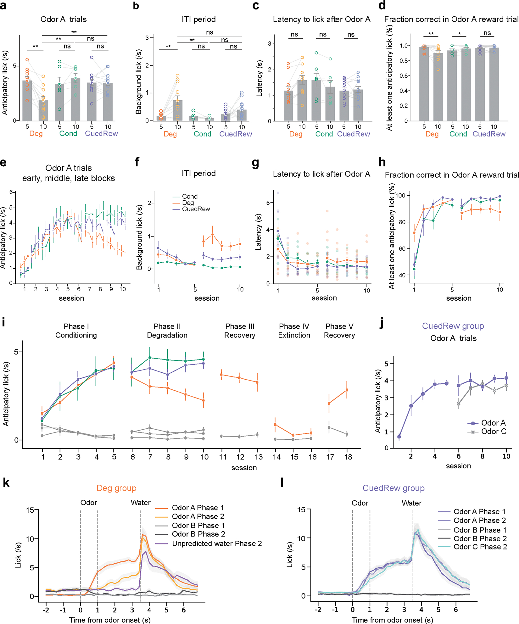
For all panels: Deg group, n = 11; Conditioning, n = 6; Cued Reward n=12. Error bars are SEM.

(a, b, c, d) Bar graphs comparing the average number of licks to Odor A during the first 3s post-stimulus (a) and during ITI (b), latency to lick (c), and fraction correct (d) in the final sessions of phase 1 and phase 2 for Deg, Cond, and CuedRew groups. Error bars represent SEM. Asterisks denote statistical significance: ns p > 0.05, **p < 0.01, paired two-sided Student’s t-test

(e) Session-wise variation in anticipatory licking for Odor A trials, broken down into early, middle, and late blocks, for all groups.

(f, g, h). Line graphs showing the average number of licks to Odor A (colored) during ITI (g), latency to lick after Odor A and fraction correct in Odor A trials for each session in the Conditioning, Degradation, and Cued Reward phase

(i) Anticipatory licking rate in Odor A trials (colored) and in Odor B trials (grey) across multiple phases: Conditioning (Phase I), Degradation (Phase II), Recovery (Phase III), Extinction (Phase IV), and post-Extinction Recovery (Phase V).

(j) Anticipatory licking to Odor C develops quickly compared to Odor A, potentially reflecting generalization.

(k, l) PSTH showing the average licking response of mice in Deg group (k) and CuedRew group (l) to the various events. The response is time-locked to the odor presentation (time 0). The shaded area indicates the standard error of the mean (SEM).

Extended Data Fig. 2 |. Dopamine responses are highly correlated across recording sites.

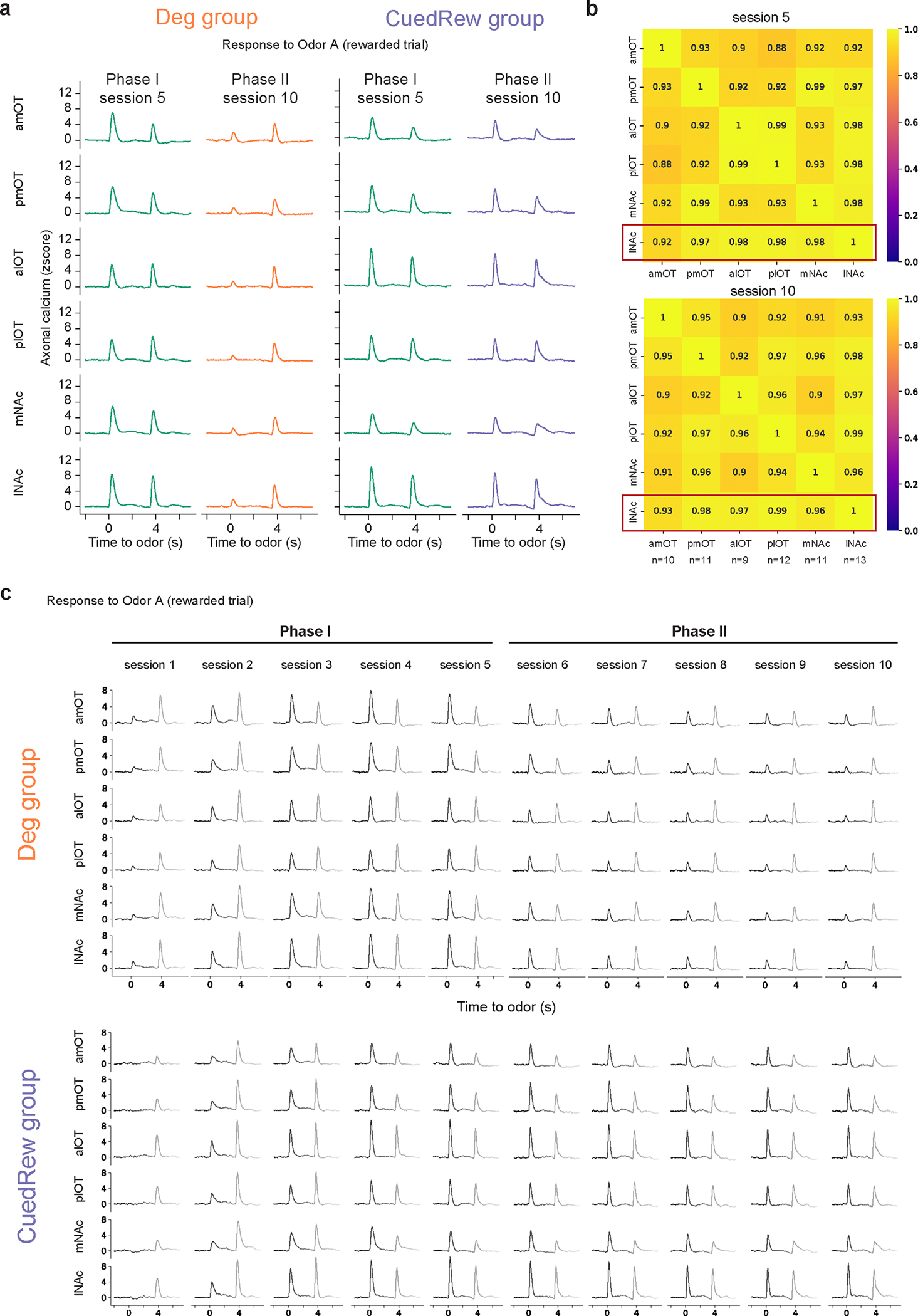
(a) Averaged dopamine axonal responses to Odor A during rewarded trials for both Deg group and CuedRew group, depicted for Phase I session 5 and Phase II session 10 across all recorded sites.

(b) Correlation matrix for averaged dopamine responses to Odor A during rewarded trials, comparing across sites from the Deg groups during sessions 5 and 10. Cosine similarity was calculated by averaging z-scored responses across trials within animals, then across animals and then computing the cosine similarity between each recording site. For some olfactory tubercule recording sites there was no discernable signal and were thus excluded from this analysis. Sample size (n) report per site.

(c) Population average dopamine responses to Odor A in rewarded trials across sessions 1 to 10 for both Deg and CuedRew groups, detailing the changes in response through Phase I and Phase II.

Extended Data Fig. 3 |. Population Average Dopamine Response per session.

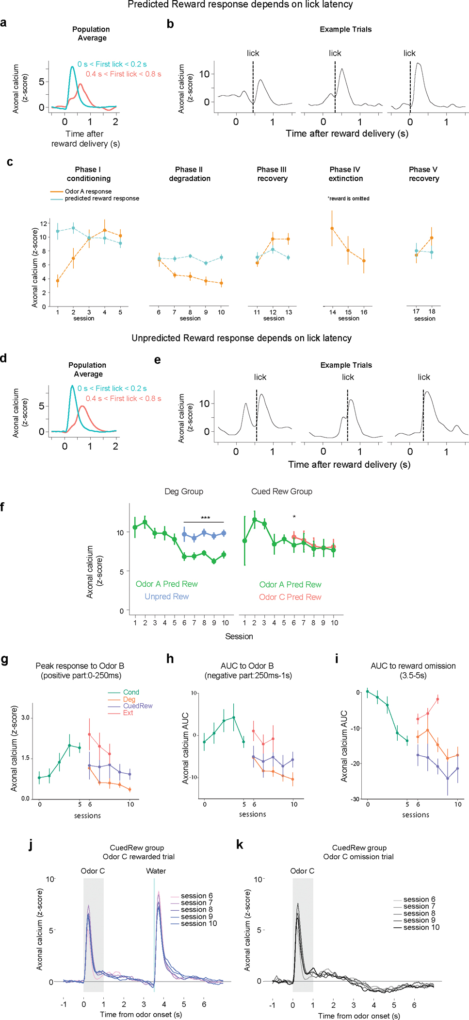
(a) Predicted reward response in Odor A trials for trials in which the first lick after reward delivery was recording within 200 ms (green) or between 400 and 800 ms (red). There is a biphasic response pattern in the slow licks, suggesting there may be sensory cues associated with reward delivery that act as conditioned stimuli

(b) Three consecutive trials from the same animal in the same session, showing the effect of lick time. The dotted line indicates the first recorded lick after reward delivery. The lick timing has an effect on the height and shape of the response.

(c) Mean peak dopamine axonal signal (z-scored) of cue response (orange) and reward response (cyan) in Odor A rewarded trial by sessions for the Deg group (n=8) across multiple phases: Conditioning (Phase I), Degradation (Phase II), Recovery (Phase III), Extinction (Phase IV), and post-Extinction Recovery (Phase V). Except in extinction, only trials in which the first lick was recorded under 250 ms was included in this analysis

(d) As in panel A, for unpredicted rewards delivered in the degradation condition.

(e) Example in three trials from the same session and animal of the response to unpredicted reward. The dotted line indicates the first recorded lick.

(f) Reward responses by session and by group. In the degradation group (n=8), the unpredicted reward elicited greater responses than the reward delivered after Odor A on all sessions (mixed-effect model, p<0.001, within animal comparison). In the Cued Rew group (n=5), the reward delivered after Odor C elicited a greater response than the reward delivered after Odor A on the first session of Cued Rew condition (two sided mixed-effect model, p<0.05, within animal comparison)

(g, h, i) Mean peak dopamine axonal signal (z-scored) across sessions for four distinct conditions, represented for various events.

(j) Response to Odor C (rewarded) and (k) Odor C (omission), population average per session

In all panels, error bars are SEM.

Extended Data Fig. 4 |. Effect of discount factor on model estimates.

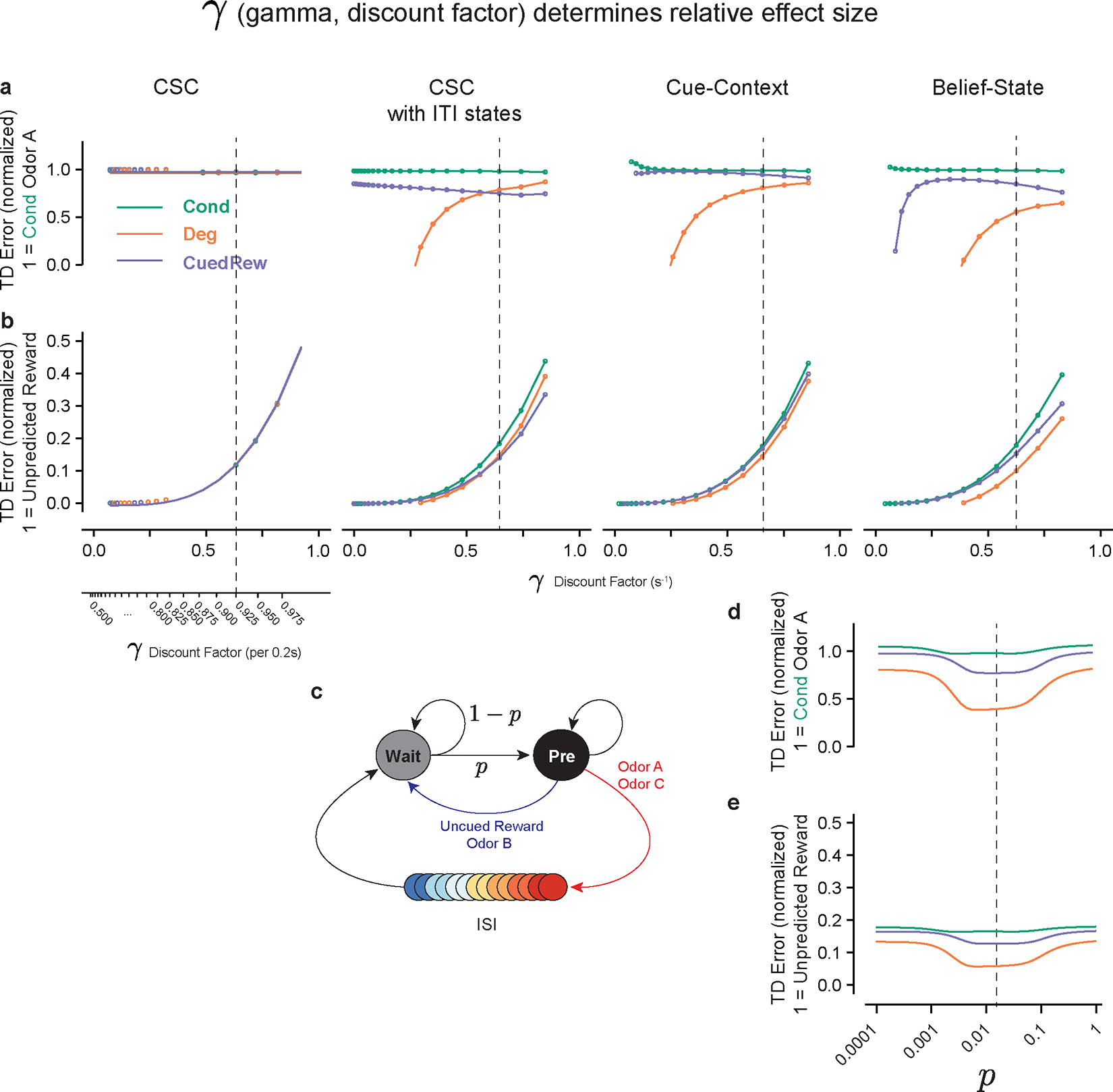
Top: Influence of discount factor (γ) on relative predicted Odor A response relative to Conditioning (a) or relative to unpredicted reward (b), where reward size = 1 for four models presented in Figure 3. Bottom left scale showing discount factor converted to step size (0.2s), other axes use per second discount. Tested range: 0.5–0.975 discount per 0.2s in 0.025 steps. Dotted line indicates discount factor used in main text.

Bottom: Effect size of transition probability in Belief-State model. The Belief-State model used assumes a fixed rate of transition (p) from the Wait state to the Pre-state with each timestep. Varying p around the value fitted to the experimental parameters has minimal effect on prediction (note logarithimic scale). If p is assumed extremely high or low than the transition from the Wait state to the Pre-state either happens almost instaneously or not at all, resulting in a single state dominating the ITI and the model behaving like the Cue-Context model.

Extended Data Fig. 5 |. Microstimuli simulation.

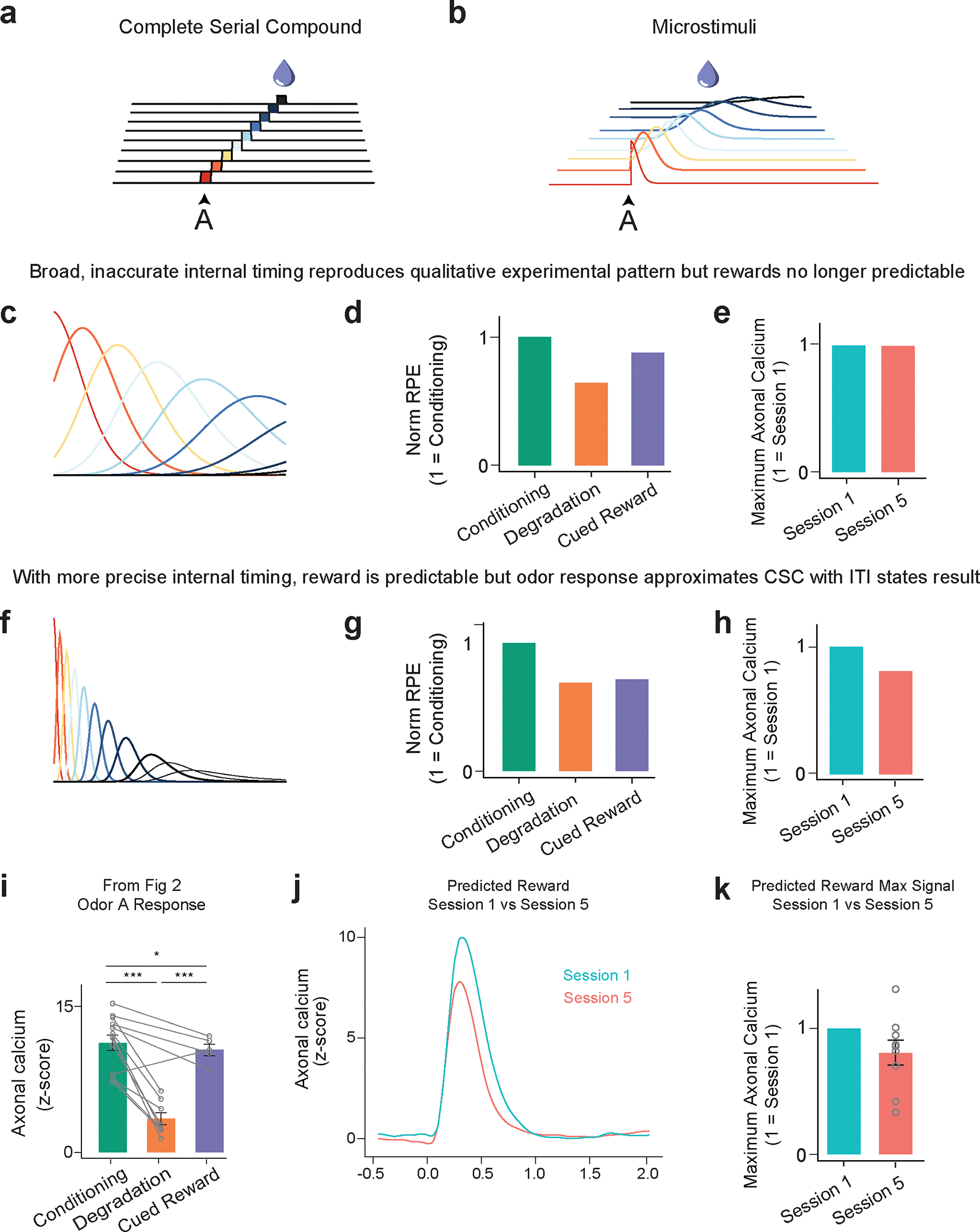
(a) Complete serial compound state spaces assume non-overlapping microstates

(b) Microstimuli state space representation assumes each stimuli produces a sequence of microstimuli that diminish in height (diminishing relative contribution) and grow in width (growing temporal imprecision).

(c) High σ and low η microstimuli simulations have low temporal precision – each state significantly overlaps with the previous

(d) With low temporal precision, microstimuli behaves like the Cue-Context model, reproducing the pattern of results qualitatively but not quantitatively.

(e) However, at this level there is no expected decrease in the predicted reward response, as the timing in insufficiently accurate.

(f) In the opposite situation, with low σ and high η, microstimuli state representations have higher precision in time

(g) However, in this case it suffers from the same issues as the CSC-with-ITI states model, predicting little difference between the Cued Reward and Degradation conditions

(h) Microstimuli help explains why the decrease in predicted reward response is not as predicted by CSC models, in which the reward is perfectly predictable (and thus the reward response following 75% reward probability cues should be 25% the magnitude of an unpredicted reward).

(i) From figure 2, mean peak dopamine axonal signal for the last session in Phase 1 (Conditioning) and 2 (Degradation and Cued Reward) for both Deg (n=8) and CuedRew (n=5) groups. Error bars represent SEM. ***, P < 0.001 in two-sided mixed-effects model with Tukey HSD posthoc.

(j) Predicted reward response following Odor A in session 1 (green) versus session 5 (red).

(k) Maximum axonal calcium response for predicted reward response following Odor A in session 1 versus session 5 (n = 13). Normalized by subject to session 1. Error bars represent SEM.

Extended Data Fig. 6 |. Comparison of reward and omission responses between experimental data, Belief-State model and value-RNN predictions.

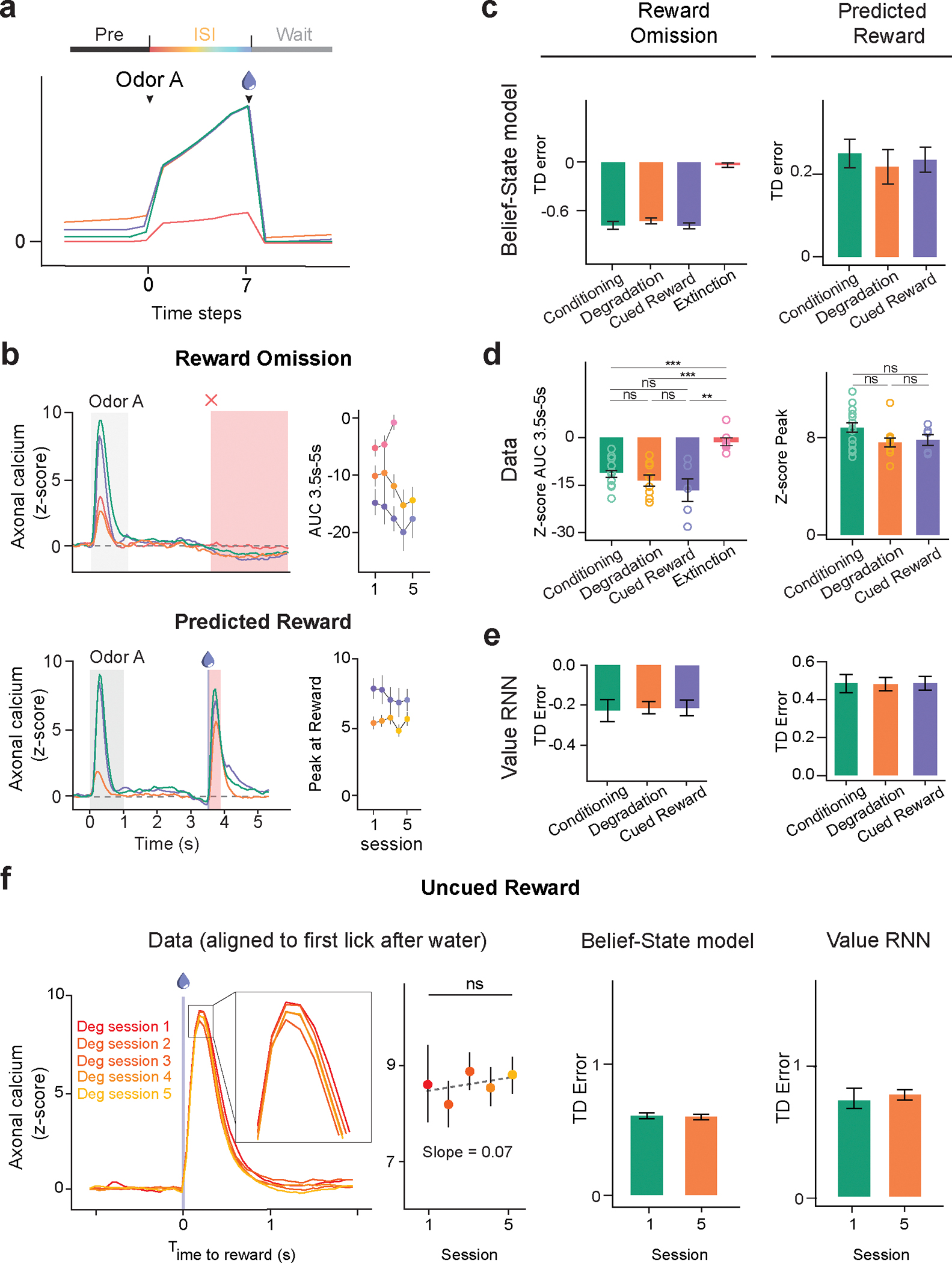
(a) Plots averaged from one representative simulation of Odor A rewarded trial (n = 4,000 simulated trials) for four distinct conditions using the Belief-State model. Graphs are for the corresponding value function of Odor A rewarded trials, with Pre state, ISI state and Wait state annotated.

(b) Z-scored DA axonal signals to reward omission and predicted reward following Odor A quantified from the red shaded area. Line graphs (right) shows mean z-scored response over multiple sessions for each condition. Statistical analysis was performed on data from the first and last session of these conditions. Error bars are SEM. ns, P > 0.05; **, P < 0.01, paired t-test.

(c) The predictions of the Belief-State model for reward omission and predicted reward (mean, error bars: SD).

(d) The experimental data for reward omission and predicted reward (mean, error bars: SEM). ns, P > 0.05; **, P < 0.01; ***, P < 0.001, Welch’s t-test.

(e) The predictions of the Value-RNN models for reward omission and predicted reward (mean, error bars: SD).

(f) The experimental data, TD error prediction by Belief-State model and Value-RNN model for uncued reward response in Degradation condition. While the Belief-State model captured the downward trend in response magnitude, none of the three statistical tests showed significant changes.

Extended Data Fig. 7 |. Methodology for visualizing state space from hidden unit activity.

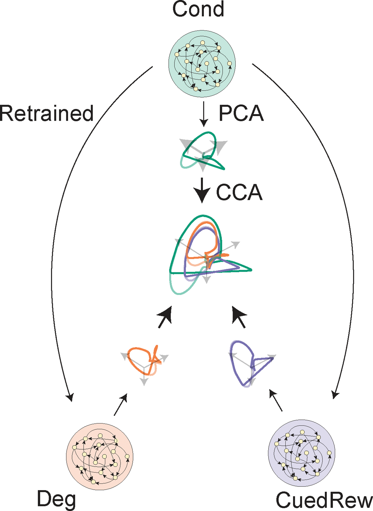
Illustration for visualizing common state space of RNN models. RNN hidden unit activity was first projected into principal component space, then canonical correlation analysis was used to align between different conditions.

Extended Data Fig. 8 |. Outcome-specific contingency degradation explained by Belief-State model and Value-RNN model.

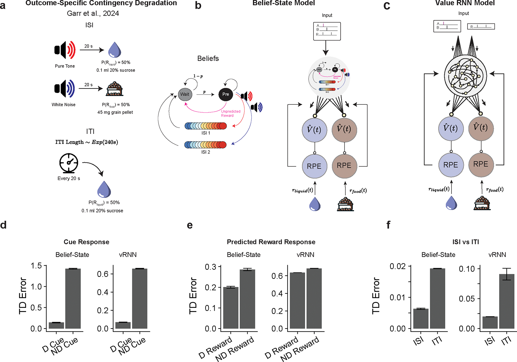
(a) Experimental design of Garr et al., two cues predicted either a liquid or food reward. During degradation, every 20 s the liquid reward was delivered with 50% probability. The ITI length was drawn from an exponential distribution with mean of 4 minutes.

(b) Belief-State model design. The Belief-State model was extended to include a second series of ISI substates to reflect the two types of rewarded trials. The model was then independently trained on the liquid reward and food reward.

(c) The value-RNN model design – as (b) but replacing the Belief-State model with the value-RNN, using a vector-valued RPE as feedback, with each channel reflecting one of the reward types.

(d-f) Summary of predicted RPE responses from Belief-State Model and Value-RNN (vRNN). The RPE was calculated as the absolute difference between the liquid RPE and food RPE. Other readout functions (e.g. weighted sum) produce similar results. Both model predictions match experimental results with degraded (D) cue (panel d) and degraded reward (e) having a reduced dopamine response versus non-degraded (ND). Furthermore, average RPE during ISI (3 seconds after cue on) and ITI (3 seconds before ITI) capture measured experimental trend. Error bars are SEM.

Data Availability

All behavioral and photometry data are available on Figshare (10.6084/m9.figshare.28216202).

References

- 1.Rescorla RA Pavlovian conditioning. It’s not what you think it is. Am Psychol 43, 151–160 (1988). [DOI] [PubMed] [Google Scholar]
- 2.Gibbon J, Berryman R & Thompson RL Contingency spaces and measures in classical and instrumental conditioning. J Exp Anal Behav 21, 585–605 (1974). [DOI] [PMC free article] [PubMed] [Google Scholar]
- 3.Hallam SC, Grahame NJ & Miller RR Exploring the edges of Pavlovian contingency space: An assessment of contingency theory and its various metrics. Learning and Motivation 23, 225–249 (1992). [Google Scholar]
- 4.Cheng PW From covariation to causation: A causal power theory. Psychological review 104, 367 (1997). [Google Scholar]
- 5.Gallistel CR, Craig AR & Shahan TA Contingency, contiguity, and causality in conditioning: Applying information theory and Weber’s Law to the assignment of credit problem. Psychol. Rev. 126, 761–773 (2019). [DOI] [PubMed] [Google Scholar]
- 6.Allan LG Human contingency judgments: rule based or associative? Psychol Bull 114, 435–448 (1993). [DOI] [PubMed] [Google Scholar]
- 7.Bermudez MA & Schultz W Responses of amygdala neurons to positive reward-predicting stimuli depend on background reward (contingency) rather than stimulus-reward pairing (contiguity). J. Neurophysiol. 103, 1158–1170 (2010). [DOI] [PMC free article] [PubMed] [Google Scholar]
- 8.Griffiths TL & Tenenbaum JB Structure and strength in causal induction. Cogn. Psychol. 51, 334–384 (2005). [DOI] [PubMed] [Google Scholar]
- 9.Gershman SJ & Ullman TD Causal implicatures from correlational statements. PLoS One 18, e0286067 (2023). [DOI] [PMC free article] [PubMed] [Google Scholar]
- 10.Papini MR & Bitterman ME The role of contingency in classical conditioning. Psychol. Rev. 97, 396–403 (1990). [DOI] [PubMed] [Google Scholar]
- 11.Kamin L Selective association and conditioning. in Fundamental issues in associative learning 42–64 (1969). [Google Scholar]
- 12.Rescorla RA & Wagner AR A Theory of Pavlovian Conditioning: Variations in the Effectiveness of Reinforcement and Nonreinforcement. in Classical conditioning II: current research and theory (eds. Black AH. & Prokasy WF.) 64–99 (1972). [Google Scholar]
- 13.Pearce JM & Bouton ME Theories of associative learning in animals. Annual review of psychology 52, 111–139 (2001). [DOI] [PubMed] [Google Scholar]
- 14.Bouton ME Learning and Behavior: A Contemporary Synthesis. (Sinauer Associates, Inc., Sunderland, MA, 2007). [Google Scholar]
- 15.Madarasz TJ et al. Evaluation of ambiguous associations in the amygdala by learning the structure of the environment. Nat. Neurosci. 19, 965–972 (2016). [DOI] [PMC free article] [PubMed] [Google Scholar]
- 16.Sutton RS & Barto AG Reinforcement Learning: An Introduction. vol. 1 (MIT Press, Cambridge, MA, 1998). [Google Scholar]
- 17.Mnih V et al. Human-level control through deep reinforcement learning. Nature 518, 529–533 (2015). [DOI] [PubMed] [Google Scholar]
- 18.Schultz W, Dayan P & Montague PR A Neural Substrate of Prediction and Reward. Science 275, 1593–1599 (1997). [DOI] [PubMed] [Google Scholar]
- 19.Cohen JY, Haesler S, Vong L, Lowell BB & Uchida N Neuron-type-specific signals for reward and punishment in the ventral tegmental area. Nature 482, 85–88 (2012). [DOI] [PMC free article] [PubMed] [Google Scholar]
- 20.Amo R et al. A gradual temporal shift of dopamine responses mirrors the progression of temporal difference error in machine learning. Nat. Neurosci. 25, 1082–1092 (2022). [DOI] [PMC free article] [PubMed] [Google Scholar]
- 21.Niv Y Reinforcement learning in the brain. Journal of Mathematical Psychology 53, 139–154 (2009). [Google Scholar]
- 22.Jeong H et al. Mesolimbic dopamine release conveys causal associations. Science 378, eabq6740 (2022). [DOI] [PMC free article] [PubMed] [Google Scholar]
- 23.Garr E et al. Mesostriatal dopamine is sensitive to changes in specific cue-reward contingencies. Sci Adv 10, eadn4203 (2024). [DOI] [PMC free article] [PubMed] [Google Scholar]
- 24.Durlach PJ Role of signals for unconditioned stimulus absence in the sensitivity of autoshaping to contingency. Journal of Experimental Psychology: Animal Behavior Processes 15, 202–211 (1989). [Google Scholar]
- 25.de Jong JW et al. A Neural Circuit Mechanism for Encoding Aversive Stimuli in the Mesolimbic Dopamine System. Neuron 101, 133–151.e7 (2019). [DOI] [PMC free article] [PubMed] [Google Scholar]
- 26.Akam T, Costa R & Dayan P Simple Plans or Sophisticated Habits? State, Transition and Learning Interactions in the Two-Step Task. PLoS Comput Biol 11, e1004648 (2015). [DOI] [PMC free article] [PubMed] [Google Scholar]
- 27.Takahashi YK et al. Expectancy-related changes in firing of dopamine neurons depend on orbitofrontal cortex. Nat. Neurosci. 14, 1590–1597 (2011). [DOI] [PMC free article] [PubMed] [Google Scholar]
- 28.Starkweather CK & Uchida N Dopamine signals as temporal difference errors: recent advances. Curr. Opin. Neurobiol. 67, 95–105 (2021). [DOI] [PMC free article] [PubMed] [Google Scholar]
- 29.Takahashi YK et al. Dopaminergic prediction errors in the ventral tegmental area reflect a multithreaded predictive model. Nat. Neurosci. 26, 830–839 (2023). [DOI] [PMC free article] [PubMed] [Google Scholar]
- 30.Daw ND, Courville AC & Touretzky DS Representation and Timing in Theories of the Dopamine System. Neural Computation 18, 1637–1677 (2006). [DOI] [PubMed] [Google Scholar]
- 31.Kobayashi S & Schultz W Influence of Reward Delays on Responses of Dopamine Neurons. J. Neurosci. 28, 7837–7846 (2008). [DOI] [PMC free article] [PubMed] [Google Scholar]
- 32.Masset P et al. Multi-timescale reinforcement learning in the brain. bioRxiv 2023.11.12.566754 (2023) doi: 10.1101/2023.11.12.566754. [DOI] [PubMed] [Google Scholar]
- 33.Ludvig EA, Sutton RS & Kehoe EJ Stimulus representation and the timing of reward-prediction errors in models of the dopamine system. Neural Comput. 20, 3034–3054 (2008). [DOI] [PubMed] [Google Scholar]
- 34.Starkweather CK, Babayan BM, Uchida N & Gershman SJ Dopamine reward prediction errors reflect hidden-state inference across time. Nat. Neurosci. 20, 581–589 (2017). [DOI] [PMC free article] [PubMed] [Google Scholar]
- 35.Starkweather CK, Gershman SJ & Uchida N The Medial Prefrontal Cortex Shapes Dopamine Reward Prediction Errors under State Uncertainty. Neuron 98, 616–629.e6 (2018). [DOI] [PMC free article] [PubMed] [Google Scholar]
- 36.Namboodiri VMK et al. Single-cell activity tracking reveals that orbitofrontal neurons acquire and maintain a long-term memory to guide behavioral adaptation. Nat. Neurosci. 22, 1110–1121 (2019). [DOI] [PMC free article] [PubMed] [Google Scholar]
- 37.Schultz W Dopamine reward prediction-error signalling: a two-component response. Nat. Rev. Neurosci. 17, 183–195 (2016). [DOI] [PMC free article] [PubMed] [Google Scholar]
- 38.Lak A, Nomoto K, Keramati M, Sakagami M & Kepecs A Midbrain Dopamine Neurons Signal Belief in Choice Accuracy during a Perceptual Decision. Curr. Biol. 27, 821–832 (2017). [DOI] [PMC free article] [PubMed] [Google Scholar]
- 39.Hennig JA et al. Emergence of belief-like representations through reinforcement learning. PLoS Comput. Biol. 19, e1011067 (2023). [DOI] [PMC free article] [PubMed] [Google Scholar]
- 40.K Namboodiri VM & Stuber GD The learning of prospective and retrospective cognitive maps within neural circuits. Neuron 109, 3552–3575 (2021). [DOI] [PMC free article] [PubMed] [Google Scholar]
- 41.van Zessen R et al. Cue and Reward Evoked Dopamine Activity Is Necessary for Maintaining Learned Pavlovian Associations. J. Neurosci. 41, 5004–5014 (2021). [DOI] [PMC free article] [PubMed] [Google Scholar]
- 42.Kalmbach A et al. Dopamine encodes real-time reward availability and transitions between reward availability states on different timescales. Nat. Commun. 13, 3805 (2022). [DOI] [PMC free article] [PubMed] [Google Scholar]
- 43.Namboodiri VMK How do real animals account for the passage of time during associative learning? Behav. Neurosci. 136, 383–391 (2022). [DOI] [PMC free article] [PubMed] [Google Scholar]
- 44.Naneix F, Marchand AR, Di Scala G, Pape J-R & Coutureau E A role for medial prefrontal dopaminergic innervation in instrumental conditioning. J Neurosci 29, 6599–6606 (2009). [DOI] [PMC free article] [PubMed] [Google Scholar]
- 45.Piquet R, Faugère A & Parkes SL A hippocampo-cortical pathway detects changes in the validity of an action as a predictor of reward. Current Biology 0, (2023). [DOI] [PubMed] [Google Scholar]
- 46.Delamater AR, Siegel DB & Tu NC Learning about reward identities and time. Behavioural Processes 207, 104859 (2023). [DOI] [PubMed] [Google Scholar]
- 47.Gallistel CR & Gibbon J Time, rate, and conditioning. Psychol. Rev. 107, 289–344 (2000). [DOI] [PubMed] [Google Scholar]
- 48.Willmore L et al. Overlapping representations of food and social stimuli in mouse VTA dopamine neurons. Neuron 111, 3541–3553.e8 (2023). [DOI] [PMC free article] [PubMed] [Google Scholar]
- 49.Millidge B, Song Y, Lak A, Walton ME & Bogacz R Reward-Bases: Dopaminergic Mechanisms for Adaptive Acquisition of Multiple Reward Types. Preprint at https://www.biorxiv.org/content/10.1101/2023.05.09.540067v1 (2023). [DOI] [PMC free article] [PubMed] [Google Scholar]
- 50.Pearl J Causality. (Cambridge university press, 2009). [Google Scholar]
- 51.Baird LC Advantage Updating. Technical report WL-TR-93–1146. Wright-Patterson Air Force Base. (1993). [Google Scholar]
- 52.Dayan P & Balleine BW Reward, motivation, and reinforcement learning. Neuron 36, 285–298 (2002). [DOI] [PubMed] [Google Scholar]
- 53.Schulman J, Moritz P, Levine S, Jordan M & Abbeel P High-Dimensional Continuous Control Using Generalized Advantage Estimation. Preprint at http://arxiv.org/abs/1506.02438 (2018). [Google Scholar]
- 54.Pan H-R, Gürtler N, Neitz A & Schölkopf B Direct Advantage Estimation. in Advances in Neural Information Processing Systems (eds. Koyejo S. et al.) vol. 35 11869–11880 (Curran Associates, Inc., 2022). [Google Scholar]
- 55.Veitch V, Wang Y & Blei DM Using embeddings to correct for unobserved confounding in networks. arXiv [stat.ML] (2019). [Google Scholar]
- 56.Rafiee B et al. From eye-blinks to state construction: Diagnostic benchmarks for online representation learning. Adapt. Behav. 31, 3–19 (2023). [DOI] [PMC free article] [PubMed] [Google Scholar]
- 57.Tomov MS, Dorfman HM & Gershman SJ Neural computations underlying causal structure learning. J. Neurosci. 38, 7143–7157 (2018). [DOI] [PMC free article] [PubMed] [Google Scholar]
- 58.Dezfouli A & Balleine BW Habits, action sequences and reinforcement learning. Eur J Neurosci 35, 1036–1051 (2012). [DOI] [PMC free article] [PubMed] [Google Scholar]
- 59.Langdon AJ, Sharpe MJ, Schoenbaum G & Niv Y Model-based predictions for dopamine. Curr. Opin. Neurobiol. 49, 1–7 (2018). [DOI] [PMC free article] [PubMed] [Google Scholar]
Methods-only references
- 60.Bäckman CM et al. Characterization of a mouse strain expressing Cre recombinase from the 3’ untranslated region of the dopamine transporter locus. Genesis 44, 383–390 (2006). [DOI] [PubMed] [Google Scholar]
- 61.Daigle TL et al. A suite of transgenic driver and reporter mouse lines with enhanced brain cell type targeting and functionality. Cell 174, 465–480.e22 (2018). [DOI] [PMC free article] [PubMed] [Google Scholar]
- 62.Kim CK et al. Simultaneous fast measurement of circuit dynamics at multiple sites across the mammalian brain. Nat. Methods (2016) doi: 10.1038/nmeth.3770. [DOI] [PMC free article] [PubMed] [Google Scholar]
- 63.Sabatini BL The impact of reporter kinetics on the interpretation of data gathered with fluorescent reporters. bioRxiv 834895 (2019) doi: 10.1101/834895. [DOI] [Google Scholar]
- 64.Gallego JA, Perich MG, Chowdhury RH, Solla SA & Miller LE Long-term stability of cortical population dynamics underlying consistent behavior. Nat Neurosci 23, 260–270 (2020). [DOI] [PMC free article] [PubMed] [Google Scholar]
- 65.Bach FR & Jordan MI Kernel independent component analysis. J. Mach. Learn. Res. 3, 1–48 (2003). [Google Scholar]
- 66.Sussillo D, Churchland MM, Kaufman MT & Shenoy KV A neural network that finds a naturalistic solution for the production of muscle activity. Nat Neurosci 18, 1025–1033 (2015). [DOI] [PMC free article] [PubMed] [Google Scholar]
- 67.Floeder JR, Jeong H, Mohebi A & Namboodiri VMK. Mesolimbic dopamine ramps reflect environmental timescales. bioRxivorg (2024) doi: 10.1101/2024.03.27.587103. [DOI] [Google Scholar]
- 68.Loewinger G, Cui E, Lovinger D & Pereira F A statistical framework for analysis of trial-level temporal dynamics in fiber photometry experiments. eLife (2024) doi: 10.7554/elife.95802.1. [DOI] [PMC free article] [PubMed] [Google Scholar]
Dataset Reference:
- Qian L et al. , Code and Data for Qian et al., 2025, Figshare, doi: 10.6084/m9.figshare.28216202, 2025 [DOI] [Google Scholar]
Associated Data
This section collects any data citations, data availability statements, or supplementary materials included in this article.
Supplementary Materials
Data Availability Statement