Macroscopic Models of Local Field Potentials and the Apparent 1/f Noise in Brain Activity

Abstract

The power spectrum of local field potentials (LFPs) has been reported to scale as the inverse of the frequency, but the origin of this 1/f noise is at present unclear. Macroscopic measurements in cortical tissue demonstrated that electric conductivity (as well as permittivity) is frequency-dependent, while other measurements failed to evidence any dependence on frequency. In this article, we propose a model of the genesis of LFPs that accounts for the above data and contradictions. Starting from first principles (Maxwell equations), we introduce a macroscopic formalism in which macroscopic measurements are naturally incorporated, and also examine different physical causes for the frequency dependence. We suggest that ionic diffusion primes over electric field effects, and is responsible for the frequency dependence. This explains the contradictory observations, and also reproduces the 1/f power spectral structure of LFPs, as well as more complex frequency scaling. Finally, we suggest a measurement method to reveal the frequency dependence of current propagation in biological tissue, and which could be used to directly test the predictions of this formalism.

Introduction

Macroscopic measurements of brain activity, such as the electroencephalogram (EEG), magnetoencephalogram or local field potentials (LFPs), display ∼1/f frequency scaling in their power spectra (1–4). The origin of such 1/f noise is at present unclear. The 1/f spectra can result from self-organized critical phenomena (5), suggesting that neuronal activity may be working according to such states (6). Alternatively, the 1/f scaling may be due to filtering properties of the currents through extracellular media (2). The latter hypothesis, however, was resting on indirect evidence, and still needs to be examined theoretically, which is one of the motivations of this article.

A continuum model (7) of LFPs incorporated the inhomogeneities of the extracellular medium into continuous spatial variations of conductivity (σ) and permittivity (ɛ) parameters. This model reproduced a form of low-pass frequency filtering in some conditions, while considering the extracellular medium as locally neutral with σ and ɛ parameters independent of frequency. This model was not entirely correct, however, because macroscopic measurements in cortex revealed a frequency dependence of electrical parameters (8). We will show here that it is possible to keep the same model structure by including plausible causes for the frequency dependence.

In a polarization model (9) of LFPs, the variations of conductivity and permittivity were considered by explicitly taking into account the presence of various cellular processes in the extracellular space around the current source. In particular, it was found that the phenomenon of surface polarization was fundamental to explain the frequency dependence of LFPs. The continuum model (7) incorporated this effect phenomenologically through continuous variations of σ and ɛ. In the polarization model, the extracellular medium is reactive in the sense that it reacts to the electric field by polarization effects. It is also locally nonneutral, which enables one to take into account the noninstantaneous character of polarization, which is at the origin of frequency dependence according to this model (9).

In this article, we propose a diffusion-polarization model that synthesizes these previous approaches and which takes into account both microscopic and macroscopic measurements. This model includes ionic diffusion, which we will show has a determinant influence on frequency filtering properties. The model also includes electric polarization, which also influences the frequency-dependent electric properties of the tissue. We show that taking into account ionic diffusion and electric polarization allows us to quantitatively account for the macroscopic measurements of electric conductivity in cortical tissue according to the experiments of Gabriel et al. (8).

However, recent measurements of Logothetis et al. (10) evidenced that the frequency dependence of cortical tissue was negligible, therefore in contradiction with the measurements of Gabriel et al. (8). We show here that the diffusion-polarization model can be consistent with both types of experiments, and thus may reconcile this contradiction. We will also examine whether this model can also explain the 1/f frequency scaling observed in LFP or EEG power spectra. Finally, we consider possible ways for experimental test of the predictions of this model.

The final goal of this approach is to obtain a model of local field potentials, which is consistent with both macroscopic measurements of conductivity and permittivity, and the microscopic features of the structure of the extracellular space around the current sources.

Materials and Methods

Numerical Simulation of Macroscopic Measurements (see Numerical Simulation of Macroscopic Measurements, below) describes the impedance of the extracellular medium based on

$$Z(r_1,\mathit{\omega })=\frac{1}{4\mathit{\pi }}{\int }_{r_1}^{\mathrm{\infty }}dr\prime \frac{1}{{r\prime }^2}\frac{1}{{\mathit{\sigma }}^{\text{M}}(r\prime ,\mathit{\omega })+i\mathit{\omega }{\mathit{\varepsilon }}^{\text{M}}(r\prime ,\mathit{\omega })}\text{.}$$ (1)

This equation gives the ω-frequency component of the impedance at point r₁ in extracellular space, in spherical symmetry (see (7) and Eq. 11 for details).

To evaluate this equation, we use MATLAB (The MathWorks, Natick, MA), which computes the Riemann sum,

$$Z(r_1,\mathit{\omega })=\frac{1}{4\mathit{\pi }}\sum _{r_1}^{\text{N}}\frac{\Delta r\prime }{{r\prime }^2}\frac{1}{{\mathit{\sigma }}^{\text{M}}(r\prime ,\mathit{\omega })+i\mathit{\omega }{\mathit{\varepsilon }}^{\text{M}}(r\prime ,\mathit{\omega })},$$ (2)

where Δr′ is the integration step (1 μm) and N is determined for a slice of 1 mm.

We also use the parametric model of Gabriel et al. (8) to simulate the frequency dependence of electrical parameters σ and ɛ of the extracellular fluid from gray matter (at a temperature of 37°C). This model is valid for frequencies included in the range of 10 Hz to 4 × 10⁸ Hz (11). According to this model, the absolute complex and macroscopic permittivity and conductivity (measured between 10 and 10¹⁰ Hz) in cortical gray matter is given by the Cole-Cole parametric model (12),

$${\mathit{\varepsilon }}_{\mathit{\omega }}^{\ast }=-i\frac{{\mathit{\sigma }}^{\ast }}{\mathit{\omega }}={\mathit{\varepsilon }}_{\mathrm{\infty }}{\mathit{\varepsilon }}_{\text{o}}+{\mathit{\varepsilon }}_{\text{o}}\sum _{\text{n}=1}^{\text{n}=4}\frac{\Delta {\mathit{\varepsilon }}_{\text{n}}}{1+{\left(i\mathit{\omega }{\tau }_{\text{n}}\right)}^{1-{\alpha }_{\text{n}}}}-i\frac{\mathit{\sigma }}{\mathit{\omega }},$$ (3)

where the sum runs over four polarization modes n, ɛ_o = 8.85 × 10⁻¹² F/m is vacuum permittivity, ɛ_∞ = 4.0 is the permittivity relative to f = 10¹⁰ Hz, σ = 0.02 S/m is the static conductivity at f = 0 Hz according to the chosen parametric model. The parameters under the sum of Eq. 3 are given in Table 1.

Table 1.

Parameter values for the parametric model of Gabriel et al. (8) (see Eq. 3)

No.	Δɛn	τn (s)	αn
1	4.50 × 101	7.96 × 10−12	0.10
2	4.00 × 102	15.92 × 10−9	0.15
3	2.0 × 105	106.1 × 10−6	0.22
4	4.5 × 107	5.305 × 10−3	0.00

Results

We start by outlining a macroscopic model with frequency-dependent electrical parameters (Macroscopic Model of Local Field Potentials), and we discuss the main physical causes for this frequency dependence (Physical Causes for Frequency-Dependent Electrical Parameters). We then constrain the model to macroscopic measurements of electrical parameters, and provide numerical simulations to test the model and reproduce the experimental observations (Numerical Simulation of Macroscopic Measurements). Finally, we propose a possible way to test the model experimentally (Measurement of Frequency Dependence).

Macroscopic model of local field potentials

In this section, we derive the equations governing the time evolution of the extracellular potential. We follow a formalism similar to the one developed previously (7), except that we reformulate the model macroscopically, to allow the electrical parameters (the conductivity σ and permittivity ɛ) to depend on frequency, as demonstrated by macroscopic measurements (8,11,13). The physical causes of this macroscopic frequency dependence will be examined in Physical Causes for Frequency-Dependent Electrical Parameters.

General formalism

We begin by deriving a general equation for the electrical potential when the electrical parameters are frequency-dependent. We start from Maxwell equations, taking the first and the divergence of the fourth Maxwell equation in a medium with constant magnetic permeability, giving

$$\begin{array}{c}\nabla \cdot \overrightarrow{D}={\mathit{\rho }}^{\text{free}}\\ \nabla \cdot \overrightarrow{j}+\frac{\partial {\mathit{\rho }}^{\text{free}}}{\partial t}=0,\end{array}$$ (4)

where $\overrightarrow{D}$, $\overrightarrow{j}$ and ρ^free are, respectively, the electric displacement, current density, and charge density in the medium surrounding the sources.

Moreover, in a linear medium the equations linking the electric field $\overrightarrow{E}$ with electric displacement $\overrightarrow{D}$, and with current density $\overrightarrow{j}$, gives

$$\overrightarrow{D}(\overrightarrow{x},t)={\int }_{-\mathrm{\infty }}^{\mathrm{\infty }}\mathit{\varepsilon }(\overrightarrow{x},\mathit{\tau })\overrightarrow{E}(\overrightarrow{x},t-\mathit{\tau })d\mathit{\tau }$$ (5)

and

$$\overrightarrow{j}(\overrightarrow{x},t)={\int }_{-\mathrm{\infty }}^{\mathrm{\infty }}\mathit{\sigma }(\overrightarrow{x},\mathit{\tau })\overrightarrow{E}(\overrightarrow{x},t-\mathit{\tau })d\mathit{\tau }\text{.}$$ (6)

The Fourier transforms of these equations are respectively ${\overrightarrow{D}}_{\mathit{\omega }}={\mathit{\varepsilon }}_{\mathit{\omega }}{\overrightarrow{E}}_{\mathit{\omega }}$ and ${\overrightarrow{j}}_{\mathit{\omega }}={\sigma }_{\mathit{\omega }}{\overrightarrow{E}}_{\mathit{\omega }}$, where we allow σ and ɛ to depend on frequency.

Given the limited precision of measurements, we can consider $\nabla \times \overrightarrow{E}\approx 0$ for frequencies <1000 Hz. Thus, we can assume that $\overrightarrow{E}=-\nabla V$, such that the complex Fourier transform of the expressions in Eq. 4 can be written as

$$\begin{array}{l}\nabla \cdot ({\mathit{\varepsilon }}_{\mathit{\omega }}\left(\overrightarrow{x}\right)\nabla V_{\mathit{\omega }})=-{\rho }_{\mathit{\omega }}^{\text{free}}\\ \nabla \cdot ({\mathit{\sigma }}_{\mathit{\omega }}\left(\overrightarrow{x}\right)\nabla V_{\mathit{\omega }})=i\mathit{\omega }{\rho }_{\mathit{\omega }}^{\text{free}}\text{.}\end{array}$$

Consequently, we have

$$\nabla \cdot (({\sigma }_{\mathit{\omega }}+\mathit{i}\mathit{\omega }{\mathit{\varepsilon }}_{\mathit{\omega }})\nabla V_{\mathit{\omega }})=\nabla ({\sigma }_{\mathit{\omega }}+\mathit{i}\mathit{\omega }{\mathit{\varepsilon }}_{\mathit{\omega }})\cdot \nabla V_{\mathit{\omega }}+({\mathit{\sigma }}_{\mathit{\omega }}+\mathit{i}\mathit{\omega }{\mathit{\varepsilon }}_{\mathit{\omega }}){\nabla }^2{V}_{\mathit{\omega }}=0\text{.}$$ (7)

Compared to previous derivations (see Eq. 49 in (7)), this equation is a more general form in which the electrical parameters can be dependent on frequency.

Macroscopic model

In principle, it is sufficient to solve Eq. 7 in the extracellular medium to obtain the frequency dependence of LFPs. However, in practice, this equation cannot be solved because the structure of the medium is too complex to properly define the limit conditions. The associated values of electric parameters must be specified for every point of space and for each frequency, which represents a considerable difficulty. One way to solve this problem is to consider a macroscopic or mean-field approach. This approach is justified here by the fact that the values measured experimentally are averaged values, which precision depends on the measurement technique. Because our goal is to simulate those measured values, we will use a macroscopic model, in which we take spatial averages of Eq. 7, and make a continuous approximation for the spatial variations of these average values. This type of approximation can be found in the classic theory of electromagnetism (15).

To this end, we define macroscopic electric parameters, ɛ^M and σ^M, as

$${\mathit{\varepsilon }}_{\mathit{\omega }}^{\text{M}}\left(\overrightarrow{x}\right)={\langle {\mathit{\varepsilon }}_{\mathit{\omega }}\left(\overrightarrow{x}\right)\rangle }_{{|}_{\text{V}}}=f(\overrightarrow{x},\mathit{\omega })$$

and

$${\mathit{\sigma }}_{\mathit{\omega }}^{\text{M}}\left(\overrightarrow{x}\right)={\langle {\mathit{\sigma }}_{\mathit{\omega }}\left(\overrightarrow{x}\right)\rangle }_{{|}_{\text{V}}}=g(\overrightarrow{x},\mathit{\omega }),$$

where V is the volume over which the spatial average is taken. We assume that V is ∼μm³, and is thus much smaller than the cortical volume, so that the mean values will be dependent of the position in cortex.

Because the average values of electric parameters are statistically independent of the mean value of the electric field, we have

$${\langle {\overrightarrow{j}}^{\text{total}}\rangle }_{{|}_{\text{V}}}(\overrightarrow{x},t)={\int }_{-\mathrm{\infty }}^{\mathrm{\infty }}{\mathit{\sigma }}^{\text{M}}\left(\mathit{\tau }\right){\langle \overrightarrow{E}\rangle }_{{|}_{\text{V}}}(\overrightarrow{x},t-\mathit{\tau })d\mathit{\tau }+{\int }_{-\mathrm{\infty }}^{\mathrm{\infty }}{\mathit{\varepsilon }}^{\text{M}}\left(\mathit{\tau }\right)\frac{\partial {\langle \overrightarrow{E}\rangle }_{{|}_{\text{V}}}}{\partial t}(\overrightarrow{x},t-\mathit{\tau })d\mathit{\tau },$$

where the first term on the right-hand side represents the dissipative contribution, and the second term represents the reactive contribution (reaction from the medium). Here, all physical effects, such as diffusion, resistive and capacitive phenomena, are integrated into the frequency dependence of σ^M and ɛ^M. We will examine this frequency dependence more quantitatively in Physical Causes for Frequency-Dependent Electrical Parameters.

The complex Fourier transform of ${\langle {\overrightarrow{j}}^{\text{total}}\rangle }_{{|}_{\text{V}}}(\overrightarrow{x},t)$ then becomes

$${\langle {\overrightarrow{j}}_{\mathit{\omega }}^{\text{total}}\rangle }_{{|}_{\text{V}}}=\left({\sigma }_{\mathit{\omega }}^{\text{M}}+i\mathit{\omega }{\mathit{\varepsilon }}_{\mathit{\omega }}^{\text{M}}\right){\langle {\overrightarrow{E}}_{\mathit{\omega }}\rangle }_{{|}_{\text{V}}}={\mathit{\sigma }}_{\text{z}}^{\text{M}}{\langle {\overrightarrow{E}}_{\mathit{\omega }}\rangle }_{{|}_{\text{V}}},$$ (8)

where σ_z^M is the complex conductivity. We can also assume

$${\mathit{\sigma }}_{\text{z}}^{\text{M}}=i\mathit{\omega }{\mathit{\varepsilon }}_{\mathrm{z}}^{\text{M}},$$ (9)

such that

$$\nabla \cdot {\langle {\overrightarrow{j}}_{\mathit{\omega }}^{\text{total}}\rangle }_{{|}_{\text{V}}}=\nabla \cdot \left({\mathit{\sigma }}_{\text{z}}^{\text{M}}{\langle {\overrightarrow{E}}_{\mathit{\omega }}\rangle }_{{|}_{\text{V}}}\right)=\nabla \cdot \left(i\mathit{\omega }{\mathit{\varepsilon }}_{\text{z}}^{\text{M}}{\langle {\overrightarrow{E}}_{\mathit{\omega }}\rangle }_{{|}_{\text{V}}}\right)=0\text{.}$$ (10)

Because σ_z^M = (σ_ω^M + iωɛ_ω^M) and ${\overrightarrow{E}}_{\mathit{\omega }}=-\nabla \langle V_{\mathit{\omega }}\rangle$, the expressions above (Eqs. 10) can also be written in the form

$$\nabla \cdot \left(({\mathit{\sigma }}_{\mathit{\omega }}^{\text{M}}+i\mathit{\omega }{\mathit{\varepsilon }}_{\mathit{\omega }}^{\text{M}})\nabla {\langle V_{\mathit{\omega }}\rangle }_{{|}_{\text{V}}}\right)=0\text{.}$$ (11)

We note that starting from the continuum model (7), where only spatial variations were considered, and generalizing this model by including frequency-dependent electric parameters, gives the same mathematical form as the original model (compare with Eq. 49 in (7)). This form invariance will allow us to introduce, in Physical Causes for Frequency-Dependent Electrical Parameters, the surface polarization phenomena by including an ad hoc frequency dependence in σ_ω^M and ɛ_ω^M. The physical causes of this macroscopic frequency dependence is that the cortical medium is microscopically nonneutral (although the cortical tissue is macroscopically neutral). Such a local nonneutrality was already postulated in a previous model of surface polarization (9). This situation cannot be accounted for by Eq. 7 if σ_ω^M and ɛ_ω^M are frequency-independent (in which case ρ_ω = 0 when ∇V_ω = 0). Thus, including the frequency dependence of these parameters enables the model to capture a much broader range of physical phenomena.

Finally, a fundamental point is that the frequency dependences of the electrical parameters σ_ω^M and ɛ_ω^M cannot take arbitrary values, but are related to each other by the Kramers-Kronig relations (17–19)

$$\Delta {\mathit{\varepsilon }}^{\text{M}}\left(\mathit{\omega }\right)=\frac{2}{\mathit{\pi }}{\int }_0^{\mathrm{\infty }}\frac{{\mathit{\sigma }}^{\text{M}}(\mathit{\omega }\prime )}{{\mathit{\omega }\prime }^2-{\mathit{\omega }}^2}d\mathit{\omega }\prime$$ (12)

and

$${\mathit{\sigma }}^{\text{M}}\left(\mathit{\omega }\right)={\mathit{\sigma }}^{\text{M}}\left(0\right)-\frac{2{\mathit{\omega }}^2}{\mathit{\pi }}{\int }_0^{\mathrm{\infty }}\frac{\Delta {\mathit{\varepsilon }}^{\text{M}}(\mathit{\omega }\prime )}{{\mathit{\omega }\prime }^2-{\mathit{\omega }}^2}d\mathit{\omega }\prime ,$$ (13)

where principal value integrals are used. These equations are valid for any linear medium (i.e., when Eqs. 5 and 6 are linear). These relations will turn out to be critical to relate the model to experiments, as we will see below.

Note that, contrary to frequency dependence, the spatial dependences of σ_ω^M and ɛ_ω^M are independent of each other, because these dependences are related to the spatial distribution of elements within the extracellular medium.

Simplified geometry for macroscopic parameters

To obtain an expression for the extracellular potential, we need to solve Eq. 11, which is possible analytically only if we consider a simplified geometry of the source and surrounding medium. The first simplification is to consider the source as monopolar. The choice of a monopolar source does not intrinsically reduce the validity of the results because multipolar configurations can be composed from the arrangement of a finite number of monopoles (20). In particular, if the physical nature of the extracellular medium determines a frequency dependence for a monopolar source, it will also do so for multipolar configurations. A second simplification will be to consider that the current source is spherical and that the potential is uniform on its surface. This simplification will enable us to calculate exact expressions for the extracellular potential and should not affect the results on frequency dependence. A third simplification is to consider the extracellular medium as isotropic. This assumption is certainly valid within a macroscopic approach, and justified by the fact that the neuropil of cerebral cortex is made of a quasirandom arrangement of cellular processes of very diverse size (21). This simplified geometry will allow us to determine how the physical nature of the extracellular medium can determine a frequency dependence of the LFPs, independently of other factors (such as more realistic geometry, propagating potentials along dendrites, etc.).

Thus, considering a spherical source embedded in an isotropic medium with frequency-dependent electrical parameters, combining with Eq. 11, we have

$$\frac{d^2{\langle V_{\mathit{\omega }}\rangle }_{{|}_{\text{V}}}}{{dr}^2}+\frac{2}{r}\frac{d{\langle V_{\mathit{\omega }}\rangle }_{{|}_{\text{V}}}}{dr}+\frac{1}{({\sigma }_{\mathit{\omega }}+i\mathit{\omega }{\mathit{\varepsilon }}_{\mathit{\omega }})}\frac{d({\mathit{\sigma }}_{\mathit{\omega }}+i\mathit{\omega }{\mathit{\varepsilon }}_{\mathit{\omega }})}{dr}\frac{d{\langle V_{\mathit{\omega }}\rangle }_{{|}_{\text{V}}}}{dr}=0\text{.}$$ (14)

Integrating this equation gives the following relation between two points r₁ and r₂ in the extracellular space,

$$r_1^2\frac{d{\langle V_{\mathit{\omega }}\rangle }_{{|}_{\text{V}}}}{dr}\left(r_1\right)\left[{\sigma }_{\mathit{\omega }}\left(r_1\right)+i\mathit{\omega }{\mathit{\varepsilon }}_{\mathit{\omega }}\left(r_1\right)\right]=r_2^2\frac{d{\langle V_{\mathit{\omega }}\rangle }_{{|}_{\text{V}}}}{dr}\left(r_2\right)\left[{\mathit{\sigma }}_{\mathit{\omega }}\left(r_2\right)+i\mathit{\omega }{\mathit{\varepsilon }}_{\mathit{\omega }}\left(r_2\right)\right]\text{.}$$ (15)

Assuming that the extracellular potential vanishes at large distances (〈V_ω〉 = 0), we find

$${\langle V_{\mathit{\omega }}\rangle }_{{|}_{\text{V}}}\left(r_1\right)=\frac{I_{\mathit{\omega }}}{4\mathit{\pi }}{\int }_{r_1}^{\mathrm{\infty }}dr\prime \frac{1}{{r\prime }^2}\frac{1}{{\sigma }_{\mathit{\omega }}(r\prime )+i\mathit{\omega }{\mathit{\varepsilon }}_{\mathit{\omega }}(r\prime )}\text{.}$$ (16)

This equation is analogous to a similar expression derived previously (Eq. 25 in (7)), but more general. The two formalisms are related by

$${\langle {\overrightarrow{j}}_{\mathit{\omega }}\rangle }_{{|}_{\text{V}}}={\mathit{\sigma }}_{\text{z}}{\langle {\overrightarrow{E}}_{\mathit{\omega }}\rangle }_{{|}_{\text{V}}}=\left({\mathrm{\sigma }}_{\mathit{\omega }}^{\text{M}}+i{\mathit{\varepsilon }}_{\mathit{\omega }}^{\text{M}}\right){\langle {\overrightarrow{E}}_{\mathit{\omega }}\rangle }_{{|}_{\text{V}}}$$

instead of ${\overrightarrow{j}}_{\mathit{\omega }}={\mathit{\sigma }}^{\text{M}}{\overrightarrow{E}}_{\mathit{\omega }}$ (see Eq. 4 in (7)). This difference is because the conductivity here depends on frequency.

In the following, we will use the simplified notations ${\overrightarrow{j}}_{\mathit{\omega }},{\overrightarrow{E}}_{\mathit{\omega }}$ and V_ω instead of ${\langle {\overrightarrow{j}}_{\mathit{\omega }}\rangle }_{{|}_{\text{V}}}$, ${\langle {\overrightarrow{E}}_{\mathit{\omega }}\rangle }_{{|}_{\text{V}}}$ and ${\langle V_{\mathit{\omega }}\rangle }_{{|}_{\text{V}}}$, respectively.

Using the relation V_ω = Z_ωI_ω, the impedance Z_ω is given by

$$Z_{\mathit{\omega }}\left(r\right)=\frac{1}{4\mathit{\pi }}{\int }_r^{\mathrm{\infty }}dr\prime \frac{1}{{r\prime }^2}\frac{1}{{\sigma }_{\mathit{\omega }}^{\text{M}}(r\prime )[1+i\mathit{\omega }{\tau }_{\mathit{\omega }}(r\prime )]},$$ (17)

where ${\tau }_{\mathit{\omega }}\left(r\prime \right)=\frac{{\mathit{\varepsilon }}_{\mathit{\omega }}^{\text{M}}}{{\sigma }_{\mathit{\omega }}^{\text{M}}}$ and r is the distance between the center of the source and the position defined by $\overrightarrow{r}$.

Physical causes for frequency-dependent electrical parameters

In the following, we successively consider two different cases of extracellular medium: first, nonreactive media, in which the current passively flows into the medium; and second, reactive media, in which some properties (such as charge distribution) may change after current flow. For each medium, we will consider two types of physical phenomena—the current produced by the electric field, and the current produced by ionic diffusion, as schematized in Fig. 1).

Figure 1.

Illustration of the two main physical phenomena involved in the genesis of local field potentials. A given current source produces an electric field, which will tend to polarize the charged membranes around the source, as schematized on the top. The flow of ions across the membrane of the source will also involve ionic diffusion to reequilibrate the concentrations. This diffusion of ions will also be responsible for inducing currents in extracellular space. These two phenomena influence the frequency filtering and the genesis of LFP signals, as explored in this article.

Nonreactive media with electric fields (Model N)

Nonreactive media ($\frac{\mathit{\omega }{\mathit{\varepsilon }}_{\mathit{\omega }}^{\text{M}}}{{\mathit{\sigma }}_{\mathit{\omega }}^{\text{M}}}\ll 1,{\mathit{\sigma }}_{\mathit{\omega }}^{\text{M}}={\mathit{\sigma }}^{\text{M}}$ and ɛ_ω^M = ɛ^M) are equivalent to resistive media, in which the resistance (or equivalently, the conductivity) does not change after the flow of current. The simplest type of such configuration consists of a resistive medium (such as a homogeneous conductive fluid) in which current sources solely interact via their electric field. Applying Eq. 17 to this configuration is equivalent to model the extracellular potential by Coulomb's law,

$$V_{\mathit{\omega }}\left(\overrightarrow{r}\right)=\frac{1}{4\mathit{\pi }{\mathit{\sigma }}^{\text{M}}}\cdot \frac{I_{\mathit{\omega }}}{r},$$ (18)

where $V_{\mathit{\omega }}\left(\overrightarrow{r}\right)$ is the extracellular potential at a position defined by $\overrightarrow{r}$ in extracellular space, and r is the absolute distance between $\overrightarrow{r}$ and the center of the current source. Here, the conductivity (σ_ω^M(r) = σ^M) is independent of space and frequency, and thus, this model is not compatible with macroscopic measurements of frequency dependence (8,11,13). It is, however, the most frequently used model to calculate extracellular field potentials (22). This model will be referred to as Model N in the following.

Nonreactive media with ionic diffusion (Model D)

Because current sources are ionic currents, there is flow of ions inside or outside of the membrane, and another physical phenomena underlying current flow is ionic diffusion. Let us consider a resistive medium such as a homogeneous extracellular conductive fluid with electric parameters

$${\mathit{\sigma }}_{\text{z}}^{\text{m}}={\sigma }_{\mathit{\omega }}^{\text{m}}\left(r\right)(1+i\frac{\mathit{\omega }{\mathit{\varepsilon }}_{\mathit{\omega }}^{\text{m}}\left(r\right)}{{\mathit{\sigma }}_{\mathit{\omega }}^{\text{m}}\left(r\right)})={\mathit{\sigma }}^{\text{m}}(1+i\frac{\mathit{\omega }{\mathit{\varepsilon }}^{\text{m}}}{{\mathit{\sigma }}^{\text{m}}})\approx {\mathit{\sigma }}^{\text{m}},$$

in which the ionic diffusion coefficient is D. When the extracellular current is exclusively due to ionic diffusion, the current density depends on frequency as $\sqrt{\mathit{\omega }}$ (see Appendices ). A resistive medium behaves as if it had a resistivity equal to $a(1+b/\sqrt{\mathit{\omega }})$, where b is complex. The parameter a is the resistivity for very high frequencies, and reflects the fact that the effect of ionic diffusion becomes negligible compared to calorific dissipation (Ohm's law) for very high frequencies. When ionic diffusion is dominant compared to electric field effects, the real part of b is much larger than a.

The frequency dependence of conductivity will be given by

$${\mathit{\sigma }}_{\mathit{\omega }}^{\text{M}}=\frac{{\mathit{\sigma }}^{\text{m}}\sqrt{\mathit{\omega }}}{\sqrt{\mathit{\omega }}+k}\text{.}$$ (19)

Applying Eq. 17 to this configuration gives the following expression for the electric potential as a function of distance:

$$V_{\mathit{\omega }}\left(\overrightarrow{r}\right)=\frac{1}{4\mathit{\pi }{\mathit{\sigma }}_{\text{z}}^{\text{M}}}\cdot \frac{I_{\mathit{\omega }}}{r}=\frac{\sqrt{\mathit{\omega }}+k}{\sqrt{\mathit{\omega }}}\cdot \frac{1}{4\mathit{\pi }{\mathit{\sigma }}^{\text{m}}}\cdot \frac{I_{\mathit{\omega }}}{r}\text{.}$$ (20)

This expression shows that, in a nonreactive medium, when the extracellular current is dominated by ionic diffusion (compared to that directly produced by the electric field), then the conductivity will be frequency-dependent and will scale as $\sqrt{\mathit{\omega }}$. This model will be referred to as Model D in the following. Note that, if the electric field primes over ionic diffusion, then we have the situation described by Model N above.

Reactive media with electric fields (Model P)

In reality, extracellular media contain different charge densities, for example due to the fact that cells have a nonzero membrane potential by maintaining differences of ionic concentrations between the inside and outside of the cell. Such charge densities will necessarily be influenced by the electric field or by ionic diffusion. As above, we first consider the case with only electric field effects and will consider next the influence of diffusion and the two phenomena taken together.

Electric polarization is a prominent type of reaction of the extracellular medium to the electric field. In particular, the ionic charges accumulated over the surface of cells will migrate and polarize the cell under the action of the electric field. It was shown previously in a theoretical study that this surface polarization phenomena can have important effects on the propagation of local field potentials (9). If a charged membrane is placed inside an electric field ${\overrightarrow{E}}_0^{\text{S}}$, there is production of a secondary electric field ${\overrightarrow{E}}_{\mathit{\omega }}^{\text{S}}$ given by (see Eq. 31 in (9))

$${\overrightarrow{E}}_{\mathit{\omega }}^{\text{S}}=\frac{{\overrightarrow{E}}_0^{\text{S}}}{1+i\mathit{\omega }{\mathit{\tau }}_{\text{M}}}\text{.}$$ (21)

This expression is the frequency-domain representation of the effect of the inertia of charge movement associated with surface polarization, reflecting the fact that the polarization does not occur instantaneously but requires a certain time to set up. This frequency dependence of the secondary electric field was derived in Bédard et al. (9) for a situation where the current was exclusively produced by electric field. The parameter τ_M is the characteristic time for charge movement (Maxwell-Wagner time) and equals ɛ^memb/σ^memb, where ɛ^memb and σ^memb are, respectively, the absolute (tangential) permittivity and conductivity of the membrane surface, respectively, and are in general very different from the permittivity and the conductivity of the extracellular fluid.

Let us now determine for zero-frequency the amplitude of the secondary field ${\overrightarrow{E}}_0^S$ produced between two cells embedded in a given electric field. First, we assume that it is always possible to trace a continuous path which links two arbitrary points in the extracellular fluid (see Fig. 2 B). Consequently, the domain defined by extracellular fluid is said to be linearly connex. In this case, the electric potential arising from a current source is necessarily continuous in the extracellular fluid. Second, in a first approximation, we can consider that the cellular processes surrounding sources are arranged randomly (by opposition to being regularly structured) and their distribution is therefore approximately isotropic. Consequently, the field produced by a given source in such a medium will also be approximately isotropic. Also consequent to this quasirandom arrangement, the equipotential surfaces around a spherical source will necessarily cut the cellular processes around the source (Fig. 2 B).

Figure 2.

Monopole and dipole arrangements of current sources. (A) Scheme of the extracellular medium containing a quasidipole (shaded) representing a pyramidal neuron, with soma and apical dendrite arranged vertically. (B) Illustration of one of the monopoles of the dipole. The extracellular space is represented by cellular processes of various size (circles) embedded in a conductive fluid. The dashed lines represent equipotential surfaces. The $\widehat{ab}$ line illustrates the fact that the extracellular fluid is linearly connex.

Suppose that at time t = 0, an excess of charge appears at a given point in extracellular space, then a static electric field is immediately produced. At this time, currents begins to flow in extracellular fluid, as well as inside the different cellular processes surrounding the source. These cells begin to polarize, with τ_MW as the characteristic polarization time. Asymptotically, the system will reach an equilibrium where the polarization will neutralize the electric field, such that there is no electric field inside the cells (zero current). Now suppose that, in the asymptotic regime, there would still be a current flowing in between cells (in the extracellular fluid); then we have two possibilities. First, the equipotential surfaces are discontinuous, or they cut the membrane surfaces (as illustrated in Fig. 2 B). The first possibility is impossible because it would imply an infinite electric field. The second possibility is also impossible, because cells are isopotential due to polarization. Therefore, we can say that, asymptotically, there is no current flowing in extracellular fluid at f = 0, and necessarily this is equivalent to a dielectric medium. In other words, a passive inhomogeneous medium with randomly distributed passive cells is a perfect dielectric at zero frequency. In this case, the conductivity must tend to 0 when frequency tends to 0. Thus, in the following, we assume that ${\overrightarrow{E}}_0^{\text{S}}=-{\overrightarrow{E}}_0^{\text{P}}$ where ${\overrightarrow{E}}_0^{\text{P}}$ is the field produced by the source.

It follows that the expression for the current density in extracellular space as a function of the electric field is given by

$${\overrightarrow{j}}_{\mathit{\omega }}={\mathit{\sigma }}_{\text{z}}^{\text{M}}{\overrightarrow{E}}_{\mathit{\omega }}^{\text{P}}={\mathit{\sigma }}^{\text{m}}\cdot (1+i\frac{{\mathit{\omega }\mathit{\varepsilon }}^{\text{m}}}{{\mathit{\sigma }}^{\text{m}}})\cdot ({\overrightarrow{E}}^{\text{P}}+{\overrightarrow{E}}^{\text{S}})={\mathit{\sigma }}^{\text{m}}\cdot (1+i\frac{{\mathit{\omega }\mathit{\varepsilon }}^{\text{m}}}{{\mathit{\sigma }}^{\text{m}}})\cdot \frac{{i\mathit{\omega }\mathit{\tau }}_{\text{M}}}{1+{i\mathit{\omega }\mathit{\tau }}_{\text{M}}}\cdot {\overrightarrow{E}}_{\mathit{\omega }}^{\text{P}}\text{.}$$

In addition, for cerebral cortical tissue, we have $1+\frac{\mathit{\omega }{\mathit{\varepsilon }}^{\text{m}}}{{\mathit{\sigma }}^{\text{m}}}\approx 1$ for frequencies >10 Hz and <1000 Hz (see (8). Thus, an excellent approximation of the conductivity can be written as

$${\mathit{\sigma }}_{\text{z}}^{\text{M}}={\mathit{\sigma }}^{\text{m}}\cdot \frac{{i\mathit{\omega }\mathit{\tau }}_{\text{M}}}{1+{i\mathit{\omega }\mathit{\tau }}_{\text{M}}}\text{.}$$ (22)

Applying Eq. 17 gives

$$V_{\mathit{\omega }}\left(\overrightarrow{r}\right)=\frac{1}{4\mathit{\pi }{\mathit{\sigma }}_{\text{z}}^{\text{M}}}\cdot \frac{I_{\mathit{\omega }}}{r}=\frac{{i\mathit{\omega }\mathit{\tau }}_{\text{M}}}{1+{i\mathit{\omega }\mathit{\tau }}_{\text{M}}}\cdot \frac{1}{4\mathit{\pi }{\mathit{\sigma }}^{\text{m}}}\cdot \frac{I_{\mathit{\omega }}}{r}\text{.}$$ (23)

This model describes the effect of polarization in reaction to the source electric field, and will be referred to as Model P in the following.

Reactive media with electric field and ionic diffusion (Model DP)

The propagation of current in the medium is dominated by ionic diffusion currents or by currents produced by the electric field, according to the values of k and k₁ with respect to $\sqrt{\mathit{\omega }}$. The values of k and k₁ are, respectively, inversely proportional to the square root of the global ionic diffusion coefficient in the extracellular fluid, and of membrane surface (see Appendices ).

We apply the reasoning based on the connex topology of the cortical medium (see above) to deduce the order of magnitude of the induced field for zero frequency ${\overrightarrow{E}}_0^{\text{S}}$,

$${\overrightarrow{E}}_{\mathit{\omega }}^{\text{S}}=-\frac{{\overrightarrow{E}}_0^{\text{P}}}{1+i\sqrt{\mathit{\omega }}\mathit{\tau }},$$ (24)

where

$$\mathit{\tau }=(\sqrt{\mathit{\omega }}+k_1){\mathit{\tau }}_{\text{M}}=\sqrt{\mathit{\omega }}\frac{{\mathit{\varepsilon }}^{\text{memb}}}{{\mathit{\sigma }}^{\text{memb}}},$$

because the tangential conductivity on membrane surface is given by

$${\sigma }_{\mathit{\omega }}^{\text{memb}}=\frac{{\mathit{\sigma }}^{\text{Memb}}\sqrt{\mathit{\omega }}}{\sqrt{\mathit{\omega }}+k_1},$$

when the current is dominated by either electric field or ionic diffusion (see Eq. 19).

It follows that the expression for the current density in extracellular space as a function of the electric field is given by

$${\overrightarrow{j}}_{\mathit{\omega }}={\mathit{\sigma }}_{\text{z}}^{\text{M}}{\overrightarrow{E}}_{\mathit{\omega }}^{\text{P}}=\frac{{\mathit{\sigma }}^{\text{m}}\sqrt{\mathit{\omega }}}{\sqrt{\mathit{\omega }}+k}\cdot (1+i\frac{\mathit{\omega }{\mathit{\varepsilon }}_{\mathit{\omega }}^{\text{m}}}{{\mathit{\sigma }}_{\mathit{\omega }}^{\text{m}}})\cdot ({\overrightarrow{E}}^{\text{P}}+{\overrightarrow{E}}^{\text{S}})\approx \frac{{\mathit{\sigma }}^{\text{m}}\sqrt{\mathit{\omega }}}{\sqrt{\mathit{\omega }}+k}\cdot \frac{i\sqrt{\mathit{\omega }}\mathit{\tau }}{1+i\sqrt{\mathit{\omega }}\mathit{\tau }}\cdot {\overrightarrow{E}}_{\mathit{\omega }}^{\text{P}},$$

because $1+i\frac{\mathit{\omega }{\mathit{\varepsilon }}_{\mathit{\omega }}^{\text{m}}}{{\mathit{\sigma }}_{\mathit{\omega }}^{\text{m}}}\approx 1$ in cortical tissue for frequencies >10 Hz and <1000 Hz (see (8)).

Thus, we have the expression for the complex conductivity of the extracellular medium,

$${\mathit{\sigma }}_{\text{z}}^{\text{M}}={\mathit{\sigma }}_{\mathit{\omega }}^{\text{M}}+i\mathit{\omega }{\mathit{\varepsilon }}_{\mathit{\omega }}^{\text{M}}=\frac{{\mathit{\sigma }}^{\text{m}}\sqrt{\mathit{\omega }}}{\sqrt{\mathit{\omega }}+k}\cdot \frac{i\sqrt{\mathit{\omega }}\mathit{\tau }}{1+i\sqrt{\mathit{\omega }}\mathit{\tau }},$$ (25)

where $\tau =(\sqrt{\mathit{\omega }}+k_1){\mathit{\tau }}_{\text{M}}$.

Thus, we have obtained a unique expression (Eq. 25) for the apparent conductivity in extracellular space outside of the source, and its frequency dependence due to differential Ohm's law, electric polarization phenomena, and ionic diffusion. These phenomena are responsible for an apparent frequency-dependence of the electric parameters, which will be compared to the frequency dependence observed in macroscopic measurements of conductivity (see Numerical Simulation of Macroscopic Measurements, below).

Finally, Eqs. 17 and 25 imply that the macroscopic impedance of a homogeneous spherical shell of width R₂–R₁ is given by

$$Z_{\mathit{\omega }}=\frac{1}{4\mathit{\pi }}{\int }_{{\text{R}}_1}^{{\text{R}}_2}\frac{1}{{r\prime }^2}\frac{dr\prime }{{\mathit{\sigma }}_{\mathit{\omega }}^{\text{M}}+i\mathit{\omega }{\mathit{\varepsilon }}_{\mathit{\omega }}^{\text{M}}}=\frac{R_2-R_1}{4\mathit{\pi }{R}_1{R}_2}\cdot \frac{1}{{\mathit{\sigma }}_{\mathit{\omega }}^{\text{M}}+i\mathit{\omega }{\mathit{\varepsilon }}_{\mathit{\omega }}^{\text{M}}}\text{.}$$ (26)

In the following, this model will be referred as the diffusion-polarization or DP model, and we will use the above expressions (Eqs. 25 and 26) to simulate experimental measurements.

Numerical simulation of macroscopic measurements

Experiments of Gabriel et al. (8,11,13)

We first consider the experiments of Gabriel et al. (8,11,13), who measured the frequency dependence of electrical parameters for a large number of biological tissues. In these experiments, the biological tissue was placed in between two capacitor plates, which were used to measure the capacitance and leak current using the relation I_ω = YV_ω, imposing the same current amplitude at all frequencies. Because the admittance value is proportional to σ_ω^M + iωɛ_ω^M, measuring the admittance provides direct information about σ_ω^M and ɛ_ω^M.

To stay coherent with the formalism developed above, we will assume that the capacitor has a spherical geometry. The exact geometry of the capacitor should, in principle, have no influence on the frequency dependence of the admittance, because the geometry will only affect the proportionality constant between σ_z and Y_ω. In the case of a spherical capacitor, by applying Eq. 26, we obtain

$$Y_{\mathit{\omega }}=\frac{1}{R}+i\mathit{\omega }C=4\mathit{\pi }\frac{R_1{R}_2}{R_2-R_1}[{\mathrm{\sigma }}_{\mathit{\omega }}^{\text{M}}+i\mathit{\omega }{\mathit{\varepsilon }}_{\mathit{\omega }}^{\text{M}}]=4\mathit{\pi }\frac{R_1{R}_2}{R_2-R_1}{\mathit{\sigma }}_{\text{z}}^{\text{M}}\text{.}$$ (27)

We also take into account the fact that the resistive part is always greater than the reactive part for low frequencies (<1000 Hz), which is expressed by

$$\mathit{\omega }{{\mathit{\varepsilon }}_{\mathit{\omega }}}^{\text{M}}/{{\sigma }_{\mathit{\omega }}}^{\text{M}}\ll 1\text{.}$$

This relation can be verified, for example, from the measurement of Gabriel et al. (8), where it is true for the whole frequency band investigated experimentally (between 10 and 10¹⁰ Hz).

The real part of σ_ω^M = σ_z then takes the form

$${\mathit{\sigma }}_{\mathit{\omega }}^{\text{M}}\approx \frac{{\mathit{\sigma }}^{\text{M}}\sqrt{\mathit{\omega }}}{\sqrt{\mathit{\omega }}+k}\cdot \frac{\mathit{\omega }{\mathit{\tau }}^2}{\mathit{\omega }{\mathit{\tau }}^2+1},$$ (28)

where $\tau =(\sqrt{\mathit{\omega }}+k_1){\mathit{\tau }}_{\text{M}}$.

By substituting this value of τ, the inverse of the conductivity (the resistivity) is given by

$$\frac{1}{{\mathit{\sigma }}_{\mathit{\omega }}^{\text{M}}}\approx \frac{1}{{\mathit{\sigma }}^{\text{M}}}\cdot \left(1+\frac{k}{\sqrt{\mathit{\omega }}}\right)\cdot \left(1+\frac{1}{\mathit{\omega }{\mathit{\tau }}_{\text{M}}^2{\left(\sqrt{\mathit{\omega }}+k_1\right)}^2}\right)=\frac{1}{{\mathit{\sigma }}^{\text{M}}}\cdot [1+\frac{k}{\sqrt{\mathit{\omega }}}+\left(\frac{1}{\mathit{\omega }{\mathit{\tau }}_{\text{M}}^2}+\frac{k}{{\mathit{\omega }}^{3/2}{\mathit{\tau }}_{\text{M}}^2}\right)\left(\frac{1}{\mathit{\omega }+2k_1\sqrt{\mathit{\omega }}+k_1^2}\right)]\text{.}$$ (29)

Finally, to reproduce the experiments of Gabriel et al., we assume $k_1\gg \sqrt{\mathit{\omega }}$. By developing in series the last term (in parentheses) of Eq. 29, we obtain

$$\frac{1}{{\mathit{\sigma }}_{\mathit{\omega }}^{\text{M}}}\approx {\overline{K}}_0+\frac{{\overline{K}}_1}{{\mathit{\omega }}^{1/2}}+\frac{{\overline{K}}_2}{\mathit{\omega }}+\frac{{\overline{K}}_3}{{\mathit{\omega }}^{3/2}}=K_0+\frac{K_1}{f^{1/2}}+\frac{K_2}{f}+\frac{K_3}{f^{3/2}}\text{.}$$ (30)

Equation 30 corresponds to the conductivity σ^M, as measured in the experimental conditions of the experiments of Gabriel et al. (the permittivity ɛ^M is obtained by applying Kramers-Kronig relations). Fig. 3 shows that this expression for the conductivity can explain the measurements in the frequency range of 10–1000 Hz, which are relevant for LFPs. To obtain this agreement, we had to assume in Eq. 25 a relatively low Maxwell-Wagner time of ∼0.15 s (f_c = 1/(2πτ_M) between 1 Hz and 10 Hz), $k_1>\sqrt{\mathit{\omega }}>k$ (for frequencies <100 Hz).

Figure 3.

Models of macroscopic extracellular conductivity compared to experimental measurements in cerebral cortex. The experimental data (labeled G) show the real part of the conductivity measured in cortical tissue by the experiments of Gabriel et al. (8). The curve labeled E represents the macroscopic conductivity calculated according to the effects of electric field in a nonreactive medium. The curve labeled D is the macroscopic conductivity due to ionic diffusion in a nonreactive medium. The curve labeled P shows the macroscopic conductivity calculated from a reactive medium with electric-field effects (polarization phenomena). The curve labeled DP shows the macroscopic conductivity in the full model, combining the effects of electric polarization and ionic diffusion. Every model was fit to the experimental data by using a least-square procedure, and the best fit is shown. The DP model's conductivity is given by Eq. 30 with K₀ = 10.84, K₁ = −19.29, K₂ = 180.35, and K₃ = 52.56. The experimental data (G) is the parametric Cole-Cole model (12), which was fit to the experimental measurements of Gabriel et al. (8). This fit is in agreement with experimental measurements for frequencies >10 Hz. No experimental measurements exist for frequencies <10 Hz, and the different curves show different predictions from the phenomenological model of Cole-Cole and these models.

This value of Maxwell-Wagner time is necessary to explain Gabriel's experiments, and may seem very large at first sight. However, the Maxwell-Wagner time is not limited by physical constraints, because we have by definition ${\mathit{\tau }}_{\text{MW}}=\frac{{\mathit{\varepsilon }}_{\mathit{\omega }}}{{\mathit{\sigma }}_{\mathit{\omega }}}$. In principle, the value of σ_ω can be very small, approaching zero, while ɛ_ω can take very large values. For example, taking the measurements of Gabriel et al. in aqueous solutions of NaCl and in gray matter (8), gives values of τ_MW comprised between 1 ms and 100 ms for frequencies at ∼10 Hz.

Thus, the model predicts that in the experiments of Gabriel et al., the transformation of electric current carried by electrons to ionic current in the biological medium necessarily implies an accumulation of ions at the plates of the capacitor. This ion accumulation will in general depend on frequency, because the conductivity and permittivity of the biological medium are frequency-dependent. This will create a concentration gradient across the biological medium, which will cause a ionic diffusion current opposite to the electric current. This ionic current will allow a greater resulting current because surface polarization is opposite to the electric field. Fig. 3 shows that such conditions give frequency-dependent macroscopic parameters consistent with the measurements of Gabriel et al.

The parameter choices to obtain this agreement can be justified qualitatively because the ionic diffusion constant on cellular surfaces is probably much smaller than in the extracellular fluid, such that k₁ ≫ k. This implies the existence of a frequency band B_f for which $\sqrt{\mathit{\omega }}$ is negligible with respect to k₁, but not with respect to k because these constants are inversely proportional to the square root of their respective diffusion coefficients. Thus, the approximation that we suggest here is that this band B_f finishes at ∼100 Hz in the experimental conditions of Gabriel et al. It is important to note that this parameter choice is entirely dependent on the ratio between ionic diffusion current and the current produced by the electric field, and thus will be depend on the particular experimental conditions.

It is interesting to note that this model and the phenomenological Cole-Cole model (12) predict different behaviors of the conductivity for low frequencies (<10 Hz). In this model, the conductivity tends to zero when frequency tends to zero, while in the Cole-Cole extrapolation, it tends to a constant value (13). The main difference between these models is that the Cole-Cole model is phenomenological and has never been deduced from physical principles for low frequencies, unlike this model, which is entirely deduced from well-defined physical phenomena.

Logothetis et al. (10) measurements

We next consider the experiments of Logothetis et al. (10), which reported a resistive medium, in contrast with the experiments of Gabriel et al. In these experiments, four electrodes were aligned and spaced by 3 mm in monkey cortex. The first and last electrodes were used to inject current, while the two intermediate electrodes were used to measure the extracellular voltage. The voltage was measured at different frequencies and current intensities.

One important point in this experimental setup is that the intensity of the current was such that the voltage at the extreme (injecting) electrodes saturates. One of the consequences of this saturation was to limit ionic diffusion effects, as discussed in Logothetis et al. (10). This voltage saturation will diminish the concentration difference near the source (we would have an amplification if this was not the case). It follows that, in the experiments of Logothetis et al., the ratio between diffusion current and electric field current is very small. Thus, in this case, we use values of parameters k_i very different from those assumed above to reproduce the experiments of Gabriel et al., in particular $k_1\ll \sqrt{\mathit{\omega }}$. As we will see in Discussion, this situation may be different from the physiological conditions.

Nevertheless, the large distance between electrodes suggests that the relation between current and voltage is linear because the current density is roughly proportional to the inverse of squared distance to the source. Consequently, we can suppose that in the experiments of Logothetis et al., the ionic gradient is negligible, which prevents ionic diffusion currents. Thus, in this experiment, most—if not all—of the extracellular current is due to electric-field effects.

In this situation, the conductivity (Eq. 25) becomes

$${\mathit{\sigma }}_{\mathit{\omega }}^{\text{M}}\approx {\mathit{\sigma }}^{\text{m}}\cdot \frac{{\left(\mathit{\omega }{\mathit{\tau }}_{\text{M}}\right)}^2}{1+{\left(\mathit{\omega }{\mathit{\tau }}_{\text{M}}\right)}^2},$$ (31)

which is similar to the Model P above.

Moreover, taking the same Maxwell-Wagner time τ_M as above for the experiments of Gabriel et al. (which corresponds to a cutoff frequency of 1 Hz), we have for frequencies >10 Hz,

$$\frac{{\left(\mathit{\omega }{\mathit{\tau }}_{\text{M}}\right)}^2}{1+{\left(\mathit{\omega }{\mathit{\tau }}_{\text{M}}\right)}^2}\approx 1,$$

similar to a resistive medium.

Thus, in the experiments of Logothetis et al., the saturation phenomenon entrains current propagation in the biological medium as if the medium was quasiresistive for frequencies >10 Hz. This constitutes a possible explanation of the contrasting results in the measurements of Logothetis et al. and Gabriel et al.

Frequency dependence of the power spectral density of extracellular potentials

The third type of experimental observation is the fact that the power spectral density (PSD) of LFPs or EEG signals displays 1/f frequency scaling (1–4). To examine whether this 1/f scaling can be accounted for by this formalism, we consider a spherical current source embedded in a continuous macroscopic medium. We also assume that the PSD of the current source is a Lorentzian, which could derive, for example, from randomly occurring exponentially decaying postsynaptic currents (2) (see Fig. 4).

Figure 4.

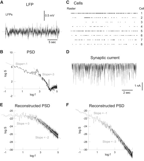
Simulation of 1/f frequency scaling of LFPs during wakefulness. (A) LFP recording in the parietal cortex of an awake cat. (B) Power spectral density (PSD) of the LFP in log scale, showing two different scaling regions with a slope of −1 and −3, respectively. (C) Raster of eight simultaneously-recorded neurons in the same experiment as in panel A. (D) Synaptic current calculated by convolving the spike trains in panel C with exponentials (decay time constant of 10 ms). (E) PSD calculated from the synaptic current, shown two scaling regions of slope 0 and −2, respectively. (F) PSD calculated using a model including ionic diffusion (see text for details). The scaling regions are of slope −1 and −3, respectively, as in the experiments in panel B. Experimental data taken from Destexhe et al. (37); see also Bédard et al. (2) for details of the analysis in panels B–D.

To simulate this situation, we used the diffusion-polarization model with ionic diffusion and electric field effects in a reactive medium. We have estimated above that surface polarization phenomena have a cutoff frequency of ∼1 Hz, and will not play a role above that frequency. So, if we focus on the PSD of extracellular potentials in the frequency range >1 Hz, we can consider only the effect of ionic diffusion (in agreement with the experiments of Gabriel et al.; see above).

Thus, we can approximate the conductivity as (see Eq. 25)

$${\mathit{\sigma }}_{\mathit{\omega }}^{\text{M}}=a\sqrt{\mathit{\omega }},$$ (32)

where a is a constant.

It follows that the extracellular voltage around a spherical current source is given by (see Eq. 17)

$$V(r,\mathit{\omega })=\frac{I_{\mathit{\omega }}}{4\mathit{\pi }a\sqrt{\mathit{\omega }}r}=\frac{V(r,1)}{\sqrt{\mathit{\omega }}}=\frac{V(R,1)R}{r\sqrt{\mathit{\omega }}},$$ (33)

where R is the radius of the source.

In other words, we can say that the extracellular potential is given by the current source I_ω convolved with a filter in $1/\sqrt{\mathit{\omega }}$, which is essentially due to ionic diffusion (Warburg impedance; see the literature (23–25).). A white noise current source will thus result in a PSD scaling as 1/f, and can explain the experimental observations, as shown in Fig. 4. Experimentally recorded LFPs in cat parietal cortex display LFPs with frequency scaling as 1/f for low frequencies, and 1/f³ for high frequencies (Fig. 4, A and B). Following the same procedure as in Bédard et al. (2), we reconstructed the synaptic current source from experimentally recorded spike trains (Fig. 4, C and D). The PSD of the current source scales as a Lorentzian (Fig. 4 E) as expected from the exponential nature of synaptic currents. Calculating the LFP around the source and taking into account ionic diffusion, gives a PSD with two frequency bands, scaling in 1/f for low frequencies, and 1/f³ for high frequencies (Fig. 4 F). This is the frequency scaling observed experimentally for LFPs in awake cat cortex (2). We conclude that ionic diffusion is a plausible physical cause of the 1/f structure of LFPs for low frequencies.

Two important points must be noted. First, the diffusion-polarization model does not automatically predict 1/f scaling at low frequencies, but rather implements an 1/f filter, which may result in frequency scaling with larger slopes. Second, the same experimental situation may result in different frequency scaling, and this is also consistent with the diffusion-polarization model. These two points are illustrated in Fig. 5, which shows a similar analysis as Fig. 4 but during slow-wave sleep in the same experiment. The LFP is dominated by slow-wave activity (Fig. 5 A), and the different units display firing patterns characterized by concerted pauses (shaded lines in Fig. 5 B), characteristic of slow-wave sleep and which are also visible in the reconstructed synaptic current (Fig. 5 C). The PSD shows a similar scaling as 1/f³ as for wakefulness, but the scaling at low frequencies is different (slope at ∼−2 at low frequencies; see Fig. 5 D). The PSD reconstructed using the diffusion-polarization model displays similar features (compare with Fig. 5 E). This analysis shows that the diffusion-polarization model qualitatively accounts for different regions of frequency scaling found experimentally in different frequency bands and network states.

Figure 5.

Simulation of more complex frequency scaling of LFPs during slow-wave sleep. (A) Similar LFP recording as in Fig. 4A (same experiment), but during slow-wave sleep. (B) Raster of eight simultaneously-recorded neurons in the same experiment as in panel A. The vertical shaded lines indicate concerted pauses of firing which presumably occur during the down states. (C) Synaptic current calculated by convolving the spike trains in panel B with exponentials (decay time constant of 10 ms). (D) Power spectral density (PSD) of the LFP in log scale, showing the same scaling regions with a slope of −3 at high frequencies as in wakefulness (the PSD in wake is shown in shading in the background). At low frequencies, the scaling was close to 1/f² (shaded line; the dotted line shows the 1/f scaling of wakefulness). (E) PSD calculated from the synaptic current in panel C, using a model including ionic diffusion. This PSD reproduces the scaling regions of slope −2 and −3, respectively (shaded lines). The low-frequency region, which was scaling as 1/f in wakefulness (dotted lines), had a slope close to −2. Experimental data taken from Destexhe et al. (37).

Measurement of frequency dependence

In this final section, we examine a possible way to test the model experimentally. The main prediction of the model is that, in natural conditions, the extracellular current perpendicular to the source is dominated by ionic diffusion. The experiments realized so far (8,10,11,13) used macroscopic currents that did not necessarily respect the correct current flow in the tissue.

We suggest creating more naturalistic current sources by generating ionic currents with a micropipette placed in the extracellular medium. By using periodic current injection during very short time Δt compared to the period (small duty cycle), we can measure, using the same electrode, the extracellular voltage V_pr (using a fixed reference far away from the source). If the period of the source is shorter than the relaxation time of the system, the voltage will integrate, which is due to charge accumulation.

Because V_pr is directly proportional to the amount of charge emitted as a function of time during Δt (capacitive effect of the extracellular medium), the time variation of V_pr is directly proportional to the ionic diffusion current. In such conditions, if the extracellular medium is purely resistive as predicted by the experiments of Logothetis et al., the relaxation time should be very small, of ∼10⁻¹² s (9), which would prevent any integration phenomena and charge accumulation for frequencies <10¹² Hz. If the medium has a slower relaxation due to polarization and ionic diffusion, then we should observe voltage integration and charge accumulation for physiological frequencies (<1000 Hz).

To illustrate the difference between these two situations, we consider the simplest case of a nonreactive medium (as in Model D above), in which the current can be produced by ionic diffusion or by the electric field, or by both. To calculate the time variations of ionic concentration and extracellular voltage, we consider the current density:

$$\overrightarrow{j}=D\nabla e\left[c\right]+\mathit{\sigma }\overrightarrow{E}\text{.}$$ (34)

According to the differential law for charge conservation and Poisson law, we have

$$\nabla \overrightarrow{j}+\frac{\partial \mathit{\rho }}{\partial t}=D{\nabla }^2\mathit{\rho }+\frac{\mathit{\sigma }}{\mathit{\varepsilon }}\mathit{\rho }+\frac{\partial \mathit{\rho }}{\partial t}=0\text{.}$$ (35)

When ionic diffusion is negligible compared to Ohm's law, we have

$$\frac{\partial \mathit{\rho }}{\partial t}+\frac{\mathit{\sigma }}{\mathit{\varepsilon }}\mathit{\rho }\approx 0\text{.}$$

It follows that the charge density is given by

$$\rho ={\rho }_{\text{o}}\exp \left(-\frac{\sigma }{\mathit{\varepsilon }}t\right)\text{.}$$ (36)

On the other hand, if ionic diffusion is the primary cause of current propagation in the extracellular medium, then the relaxation time should be much larger and thus, integration should be observed. When ionic diffusion is dominant, we have

$$\frac{\partial \mathit{\rho }}{\partial t}+D{\nabla }^2\mathit{\rho }\approx 0$$

instead of Eq. 35.

The general solution is

$$\mathit{\rho }=\frac{1}{\sqrt{2Dt}}{\int }_0^{\mathrm{\infty }}\mathit{\rho }(r,0)e^{-\frac{-r^2}{4Dt}}dr\text{.}$$ (37)

The difference between the expressions above (Eqs. 36 and 37) shows that the time variation of charge density is different according to which current dominates, electric field current or ionic diffusion current. The same applies to the electric potential between the electrode and a given reference, because this potential is linked to charge density through Poisson's law. Therefore, this experiment would be crucial to clearly show which of the two currents primes for currents perpendicular to the source (this would not apply to longitudinal currents, like axial currents in dendrites). In the hypothetical case of dominant ionic diffusion, the cortex would be similar to a Warburg impedance and one can estimate the macroscopic diffusion coefficient using Eq. 37.

Thus, using a micropipette injecting periodic current pulses, it should be possible to test the capacity of the medium to create charge accumulation for physiological frequencies. If this is the case, it would constitute evidence that ionic currents are nonnegligible in the physiological situation.

Discussion

In this article, we have proposed a framework to model local field potentials, and which synthesizes previous measurements and models. This framework integrates microscopic measurements of electric parameters (conductivity σ and permittivity ɛ) of extracellular fluids, with macroscopic measurements of those parameters (σ_ω^M, ɛ_ω^M) in cortical tissue (8,10). It also integrates previous models of LFPs, such as the continuum model (7), which was based on a continuum hypothesis of electric parameters variations in extracellular space, or the polarization model (9), which explicitly considered different media (fluid and membranes) and their polarization by the current sources. This model is more general and also integrates ionic diffusion, which is predicted as a major determinant of the frequency dependence of LFPs. This diffusion-polarization model also accounts for observations of 1/f frequency scaling of LFP power spectra, which is due here to ionic diffusion, and is therefore predicted to be a consequence of the genesis of the LFP signal, rather than being solely due to neuronal activity (see (2)). Finally, this work suggests that emphatic interactions between neurons can occur not only through electric fields but that ionic diffusion should also be considered in such interactions.

As discussed in Simplified Geometry for Macroscopic Parameters, this model rests on several approximations, which were necessary to obtain the analytic expressions used here. These approximations were that current sources were considered as monopolar entities (longitudinal currents such as axial currents in dendrites were not taken into account), the current source was spherical and the extracellular medium was considered isotropic. Because multipolar effects can be reconstructed from the superposition of monopoles (20), the monopolar configuration should not affect the results on frequency dependence, as long as the extracellular current perpendicular to the source is considered. Similarly, the exact geometry of the current source should have no influence on the frequency dependence far away from the sources. However, in the immediate vicinity of the sources, the geometric nature and the synchrony of synaptic currents can have influences on the power spectrum (26). Another assumption is that the extracellular medium is isotropic, which was justified within the macroscopic framework followed here. These factors, however, will influence the exact shape of the LFPs. More quantitative models including a more sophisticated geometry of current sources and the presence of membrane excitability and action potentials should be considered (e.g., (26,27)).

The main prediction of this model is that ionic diffusion is an essential physical cause for the frequency dependence of LFPs. We have shown that the presence of ionic diffusion allows the model to account quantitatively for the macroscopic measurements of the frequency dependence of electric parameters in cortical tissue (8). Ionic diffusion is responsible for a frequency dependence of the impedance as $1/\sqrt{\mathit{\omega }}$ for low frequencies (<1000 Hz), which directly accounts for the observed 1/f frequency scaling of LFP and EEG power spectra during wakefulness (1–4) (see Fig. 4). Note that the EEG is more complex because it depends on the diffusion of electric signals across fluids, dura matter, skull, muscles, and skin. However, this filtering is of low-pass type, and may not affect the low-frequency band, so there is a possibility that the 1/f scaling of EEG and LFPs have a common origin. This model is consistent with the view that this apparent 1/f noise in brain signals is not generated by self-organized features of brain activity, but is rather a consequence of the genesis of the signal and its propagation through extracellular space (2).

It is important to note that the fact that ionic diffusion may be responsible for 1/f frequency scaling of LFPs is not inconsistent with other factors, which may also influence frequency scaling. For example, the statistics of network activity—and more generally network state—can affect frequency scaling. This is apparent when comparing awake and slow-wave sleep LFP recordings in the same experiment, showing that the 1/f scaling is only seen in wakefulness but 1/f² scaling is instead seen during sleep (2) (see Fig. 5). In agreement with this, recent results indicate that the correlation structure of synaptic activity may influence frequency scaling at the level of the membrane potential, and that correlated network states scale with larger (more negative) exponents (28).

We also investigated ways to explain the measurements of Logothetis et al. (10), who reported that the extracellular medium was resistive and therefore did not display frequency dependence, in contradiction with the measurements of Gabriel et al. (8). We summarize and discuss our conclusions below.

In the experiments of Gabriel et al. (8), one measures permittivity and conductivity in the medium in between two metal plates. This forms a capacitor, which (macroscopic) complex impedance is measured. This measure actually consists of two independent measurements, the real and imaginary part of the impedance. These values are used to deduce the macroscopic permittivity and macroscopic conductivity of the medium. However, at the interface between the medium and the metal plates, the flow of electrons in the metal corresponds to a flow of charges in the tissue, and a variety of phenomena can occur, which can interfere with the measurement. The accumulation of charges that occurs at the interface between the electrode and the extracellular fluid implies a polarization impedance, which depends on the interaction between ions and the metal plate. Because this accumulation of charge implies a variation of concentration, the flow of ions may involve an important component of ionic diffusion.

In the experiments of Logothetis et al., a system of four electrodes is used; the two extreme electrodes inject current in the medium, while the two electrodes in the middle are exclusively used to measure the voltage. This system is supposed to be more accurate than Gabriel's, because the electrodes that measure voltage are not subject to charge accumulation. However, the drawback of this method are nonlinear effects. The magnitude of the injected current is such that the voltage at the extreme electrodes saturates. This voltage saturation also implies saturation of concentration (capacitive effect between electrodes), which limits ionic diffusion currents. Thus, the ratio between ionic diffusion currents and the currents due to the electric field is greatly diminished relative to the experiments of experiments of Gabriel et al.

We think that natural current sources are closer to the situation of Gabriel et al. for several reasons. First, the magnitude of the currents produced by biological sources is far too low for saturation effects. Second, the flow of charges across ion channels will produce perturbations of ionic concentration, which will be reequilibrated by diffusion. The effects may not be as strong as the perturbations of concentrations induced by the experiments of Gabriel et al., but ionic diffusion should play a role in both cases. This is precisely one of the aspects that should be evaluated in further experiments.

The experiments of Logothetis et al. were done using a four-electrode setup, which neutralizes the influence of electrode impedance on voltage measurements (29,30). This system was used to perform high-precision impedance measurements, also avoiding ionic diffusion effects (10). Indeed, these experimental conditions, and the apparent resistive medium, could be reproduced by this model if ionic diffusion was neglected. This model therefore formulates the strong prediction that ionic diffusion is important, and that any measurement technique should allow ionic diffusion to reveal the correct frequency-dependent properties of impedance and electric parameters in biological tissue.

The critical question that remains to be solved is whether, in physiological conditions, ionic diffusion plays a role as important as suggested here. We propose a simple method to test this hypothesis. The frequency dependence could be evaluated by using an extracellular electrode injecting current in conditions as close as possible to physiological conditions (a micropipette would be appropriate). By measuring the integration of the extracellular voltage after periodic current injection, one could estimate the relaxation time of the medium with respect to charge accumulation. If this relaxation time occurs at timescales relevant to neuronal currents (milliseconds) rather than the fast relaxation predicted by a purely resistive medium (picoseconds), then ionic diffusion will necessarily occur in physiological conditions, which would provide evidence in favor of this mechanism.

Appendix A: Estimation of Ionic Diffusion Current Versus Electric Diffusion In Sea Water and In Cortex

In this Appendix, we evaluate the ratio between ionic diffusion currents and electric field currents in the extracellular space directly adjacent to the source. This ratio measures whether the ionic diffusion current perpendicular to the membrane is greater than the electric field current. We will design this ratio by the term r_ie.

We have in general

$${\overrightarrow{j}}_{\text{Total}}=eD\nabla \left[\text{C}\right]+\mathit{\sigma }\nabla V,$$ (38)

where the first term on the right-hand side is the electric current density produced by ionic diffusion, and the second term is that produced by differential Ohm's law.

For a displacement Δr = 10 nm in the direction across the membrane (from inside to outside), we have approximatively

$${\overrightarrow{j}}_{\text{Total}}\cdot d\overrightarrow{r}\simeq {\overrightarrow{j}}_{\text{Total}}\cdot \overrightarrow{\Delta }r=e\Delta {\left[\text{C}\right]}_{\Delta r=10\text{nm}}+{\mathit{\sigma }}_{\mathit{\omega }}\Delta V_{\Delta r=10\text{nm}}\text{.}$$ (39)

Suppose that we have a spherical cell of 10-μm radius, embedded in sea water and at resting potential. The resting membrane potential is a dynamic equilibrium between inflow and outflow of charges, in which these two fluxes are equal on (temporal) average. Fluctuations of current around this average in the extracellular medium around the membrane have all characteristics of thermal noise (31) because the shot noise (see (16,32)) is zero when the current is zero on average, such that the net charge on the external side of the membrane varies around a mean value with the same characteristics as white noise (thermal noise). These fluctuations will therefore be present also at the level of the membrane potential. In this Appendix, we evaluate the order of magnitude of the electric current caused by ionic diffusion, relative to the electric field for this situation of dynamic equilibrium.

First, the ratio between the membrane voltage noise and the variation of total charge concentration is given by

$$\Delta Q_{\text{tot}}=C\Delta V_{\text{membrane}}=k_1\Delta V_{\text{membrane}}=1.25\times {10}^{-11}\Delta V_{\text{membrane}},$$ (40)

because the cell's capacitance is given by C = 4πR²C_m = 0.04πR² (C_m ≃ 10⁻² F/m²).

Second, mass conservation imposes

$$\Delta Q_{\text{tot}}=e^{\ast }{v}_{\text{eff}}^{\ast }\Delta {\left[C\right]}_{\text{tot}},$$ (41)

where e = 1.69 × 10⁻¹⁹ C and v_eff is the volume of the spherical shell containing the charges. Because the charges are not uniformly distributed inside the cell, but rather distributed within a thin spherical shell adjacent to the membrane, because the electric field developed across the membrane is very intense (of ∼$\frac{70\times {10}^{-3}}{7\times {10}^{-9}}$ = V/m = 10⁷ V/m). Thus, the width of the shell is ∼$dR\simeq {10}^{-4}R<1\text{nm}$, where the volume of the spherical shell is approximately equal to 4πR²dR. In this case, we have for monovalent ions (|z| = 1)

$$\Delta Q_{\text{tot}}=k_2\Delta {\left[\text{C}\right]}_{\text{tot}}\simeq 2.2\times {10}^{-38}\Delta {\left[\text{C}\right]}_{\text{tot}}=2.2\times {10}^{-38}\Delta {\left[\text{C}\right]}_{\Delta r=10\text{nm}}$$ (42)

if we assume that the variation of concentration on the adjacent border of the exterior surface of the cell is within a width of 10 nm.

In this case, we have

$$\frac{\Delta {\left[C\right]}_{\Delta r=10\text{nm}}}{\Delta V_{\text{membrane}}}=\frac{k_1}{k_2}\simeq {10}^{27}C/m^{3}V\text{.}$$ (43)

Third, the potential difference between the cell surface and 10 nm away from it, is given by

$$\Delta V_{\Delta r=10\text{nm}}=\Delta V_{\text{membrane}}-\frac{R\Delta V_{\text{membrane}}}{R+r}\simeq {10}^{-3}\Delta V_{\text{membrane}}\text{.}$$ (44)

Consequently, the ratio between ionic diffusion current and electric diffusion current caused by thermal noise in sea water obeys

$$r_{\text{ie}}\approx \frac{e{D}_{\text{sea}}\Delta {\left[C\right]}_{\Delta r=10\text{nm}}\Delta t}{{\mathit{\sigma }}_{\mathit{\omega }}^{\text{sea}}\Delta V_{\Delta r=10\text{nm}}}=\frac{e{D}_{\text{sea}}{k}_1}{{\mathit{\sigma }}_{\mathit{\omega }}^{\text{sea}}{k}_2}\simeq \frac{{10}^2}{{\mathit{\sigma }}_{\mathit{\omega }}^{\text{sea}}},$$ (45)

where the diffusion constant of K⁺ or Na⁺ in sea water is ∼${10}^{-9}\frac{{\text{m}}^2}{\text{s}}$. This implies that the ratio r is ≫1 for frequencies <1000 Hz because σ_ω^sea of sea water is necessarily <2 S/m.

Because tortuosity is given by $\lambda =\sqrt{D_{\text{sea}}/D_{\text{cortex}}}$, and is comprised between 1.6 and 2.2 (for small and large molecules, respectively) in cerebral cortex (33–35), the macroscopic diffusion constant in cortex is certainly larger than D_sea/10. Thus, we have

$$r_{\text{ie}}^{\text{cortex}}>\frac{10}{{\mathit{\sigma }}_{\mathit{\omega }}^{\text{cortex}}}$$ (46)

where ${\mathit{\sigma }}_{f=100\text{Hz}}^{\text{cortex}}$ ≃ 0.1 S/m (see (11)).

This evaluation shows that the phenomenon of ionic diffusion is essential to determine the current field in the cortex.

Finally, we note that we did not need to evaluate the absolute magnitude of ΔV in our evaluation. This evaluation is valid for a physical situation where we have a permanent white noise over a distance of 10 nm, independently of the intensity of this noise (which in practice will depend on many factors, such as the size of the cell, the number of ion channels, etc).

Appendix B: Frequency Scaling of Ionic Diffusion

In this Appendix, we calculate the frequency dependence of ionic diffusion current outside of a spherical current source. We consider a constant variation of ionic concentration, ΔX_i, on the surface of the source, and a null variation at an infinite distance (Warburg conditions).

The diffusion equation for a given ionic species is

$$\frac{\partial \Delta X_{\text{i}}}{\partial t}=D_{\text{i}}{\nabla }^2\Delta X_{\text{i}},$$ (47)

where ΔX_i is the perturbation of concentration X_i of ion i around the steady-state value, and D_i is the associated diffusion coefficient. This diffusion coefficient depends of the ionic species considered and the structure of the medium.

Because the geometry of the problem and the limit conditions respect spherical symmetry, we use spherical coordinates. In this coordinate system, we have

$$\frac{\partial \Delta X_{\text{i}}}{\partial t}=D_{\text{i}}\left[\frac{{\partial }^2\Delta X_{\text{i}}}{\partial r^2}+\frac{2}{r}\frac{\partial \Delta X_{\text{i}}}{\partial r}\right]$$ (48)

because ΔX_i does not depend on θ and of Φ (spherical symmetry).

The Fourier transform of ΔX_i with respect to time gives

$$\frac{{\partial }^2{X}_{{\text{i}}_{\mathit{\omega }}}}{\partial r^2}+\frac{2}{r}\frac{\partial \Delta X_{{\text{i}}_{\mathit{\omega }}}}{\partial r}=\frac{d^2{X}_{{\text{i}}_{\mathit{\omega }}}}{d{r}^2}+\frac{2}{r}\frac{d\Delta X_{{\text{i}}_{\mathit{\omega }}}}{dr}=\frac{i\mathit{\omega }}{D_{\text{i}}}\Delta X_{{\text{i}}_{\mathit{\omega }}},$$ (49)

which general solution is given by

$$\Delta X_{{\text{i}}_{\mathit{\omega }}}=A\left(\mathit{\omega }\right)\frac{e^{\sqrt{\frac{\text{i}\mathit{\omega }}{D_{\text{i}}}}r}}{r}+B\left(\mathit{\omega }\right)\frac{e^{-\sqrt{\frac{\text{i}\mathit{\omega }}{D_{\text{i}}}}r}}{r}\text{.}$$ (50)

For a variation of concentration at the source border which is independent of frequency and which satisfies the Warburg hypothesis (the variation of concentration tends to zero at an infinite distance (23,36)), we have

$$\Delta X_{{\text{i}}_{\mathit{\omega }}}\left(r\right)=\Delta X_{{\text{i}}_{\mathit{\omega }}}\left(R\right)\cdot \frac{R{e}^{-\sqrt{\frac{\text{i}\mathit{\omega }}{D_{\text{i}}}}(r-R)}}{r},$$ (51)

where r is the distance between the center of the source and R is the radius of the source.

Thus, the electric current density produced by ionic diffusion is given by

$${\overrightarrow{j}}_{\text{i}}\left(r\right)=Ze{D}_{\text{i}}\frac{\partial \Delta X_{\text{i}}}{\partial r}\widehat{r}=-Ze{D}_{\text{i}}(\frac{1}{r}+\sqrt{\frac{i\mathit{\omega }}{D_{\text{i}}}})\Delta X_{{\text{i}}_{\mathit{\omega }}}\left(r\right)\widehat{r},$$ (52)

where Ze is the charge of ions i.

Because we can consider that the source and extracellular medium form a spherical capacitor, the voltage difference between the surface of the source and infinite distance is given by $ZeC\Delta X_{{\text{i}}_{\mathit{\omega }}}\left(R\right)$, where C is the capacitance value. Thus, the electric impedance of the medium is given by

$$Z_{\mathit{\omega }}=\frac{C}{D_{\text{i}}(\frac{1}{R}+\sqrt{\frac{\text{i}\mathit{\omega }}{D_{\text{i}}}})}\text{.}$$ (53)

For a source of radius R = 10 μm and a macroscopic ionic diffusion coefficient of ∼10⁻¹¹ m²/s, and for frequencies >1 Hz, we can approximate the impedance by

$$Z_{\mathit{\omega }}\approx \frac{C}{\sqrt{i\mathit{\omega }{D}_{\text{i}}}}\text{.}$$ (54)

The same expression for the impedance is also obtained in cylindrical coordinates or planar Cartesian coordinates (not shown).

Note that if several ionic species are present, then the superposition principle applies (Fick equations are linear) and therefore the contribution of each ion will add up. The diffusion constants for different ions are of the same order of magnitude (for Na⁺, K⁺, Cl⁻, Ca²⁺), so no particular ion would be expected to dominate.

References

- 1.Bhattacharya J., Petsche H. Universality in the brain while listening to music. Proc. Biol. Sci. 2001;268:2423–2433. doi: 10.1098/rspb.2001.1802. [DOI] [PMC free article] [PubMed] [Google Scholar]
- 2.Bédard C., Kröger H., Destexhe A. Does the 1/f frequency scaling of brain signals reflect self-organized critical states? Phys. Rev. Lett. 2006;97:118102. doi: 10.1103/PhysRevLett.97.118102. [DOI] [PubMed] [Google Scholar]
- 3.Novikov E., Novikov A., Shannahoff-Khalsa D., Schwartz B., Wright J. Scale-similar activity in the brain. Phys. Rev. E Stat. Phys. Plasmas Fluids Relat. Interdiscip. Topics. 1997;56:R2387–R2389. [Google Scholar]
- 4.Pritchard W.S. The brain in fractal time: 1/f-like power spectrum scaling of the human electroencephalogram. Int. J. Neurosci. 1992;66:119–129. doi: 10.3109/00207459208999796. [DOI] [PubMed] [Google Scholar]
- 5.Jensen H.J. Cambridge University Press; Cambridge, UK: 1998. Self-Organized Criticality: Emergent Complex Behavior in Physical and Biological Systems. [Google Scholar]
- 6.Beggs J., Plenz D. Neuronal avalanches in neocortical circuits. J. Neurosci. 2003;23:11167–11177. doi: 10.1523/JNEUROSCI.23-35-11167.2003. [DOI] [PMC free article] [PubMed] [Google Scholar]
- 7.Bédard C., Kröger H., Destexhe A. Modeling extracellular field potentials and the frequency-filtering properties of extracellular space. Biophys. J. 2004;86:1829–1842. doi: 10.1016/S0006-3495(04)74250-2. [DOI] [PMC free article] [PubMed] [Google Scholar]
- 8.Gabriel S., Lau R.W., Gabriel C. The dielectric properties of biological tissues: II. Measurements in the frequency range 10 Hz to 20 GHz. Phys. Med. Biol. 1996;41:2251–2269. doi: 10.1088/0031-9155/41/11/002. [DOI] [PubMed] [Google Scholar]
- 9.Bédard C., Kröger H., Destexhe A. Model of low-pass filtering of local field potentials in brain tissue. Phys. Rev. E Stat. Nonlin. Soft Matter Phys. 2006;73:051911. doi: 10.1103/PhysRevE.73.051911. [DOI] [PubMed] [Google Scholar]
- 10.Logothetis N.K., Kayser C., Oeltermann A. In vivo measurement of cortical impedance spectrum in monkeys: implications for signal propagation. Neuron. 2007;55:809–823. doi: 10.1016/j.neuron.2007.07.027. [DOI] [PubMed] [Google Scholar]
- 11.Gabriel S., Lau R.W., Gabriel C. The dielectric properties of biological tissues: III. Parametric models for the dielectric spectrum tissues. Phys. Med. Biol. 1996;41:2271–2293. doi: 10.1088/0031-9155/41/11/003. [DOI] [PubMed] [Google Scholar]
- 12.Cole K.S., Cole R.H. Dispersion and absorption in dielectrics. I. Alternating current characteristics. J. Chem. Phys. 1941;9:341–351. [Google Scholar]
- 13.Gabriel S., Lau R.W., Gabriel C. The dielectric properties of biological tissues: I. Literature survey. Phys. Med. Biol. 1996;41:2231–2249. doi: 10.1088/0031-9155/41/11/001. [DOI] [PubMed] [Google Scholar]
- 14.Berg H.C. Princeton University Press; Princeton: 1983. Random Walks in Biology. [Google Scholar]
- 15.Maxwell J.C. A Treatise on Electricity and Magnetism. Vol. 1. Clarendon Press; Oxford, UK: 1873. [Google Scholar]
- 16.Buckingham M.J.J. John Wiley & Sons; New York: 1985. Noise in Electronic Devices and Systems. [Google Scholar]
- 17.Foster K.R., Schwan H.P. Dielectric properties of tissues and biological materials: a critical review. Crit. Rev. Biomed. Eng. 1989;17:25–104. [PubMed] [Google Scholar]
- 18.Kronig R.D.L. On the theory of dispersion of x-rays. J. Opt. Soc. Am. 1926;12:547–556. [Google Scholar]
- 19.Landau L.D., Lifshitz E.M. Pergamon Press; Moscow, Russia: 1984. Electrodynamics of Continuous Media. [Google Scholar]
- 20.Purcell E.M. McGraw Hill; New York: 1984. Electricity and Magnetism. [Google Scholar]
- 21.Braitenberg V., Shutz A. 2nd Ed. Springer-Verlag; Berlin, Germany: 1998. Cortex: Statistics and Geometry of Neuronal Connectivity. [Google Scholar]
- 22.Nunez P.L., Novikov A., Srinivasan R. 2nd Ed. Oxford University Press; Oxford, UK: 2006. Electric Fields of the Brain. [Google Scholar]
- 23.Diard J.-P., Le Gorrec B., Montella C. Linear diffusion impedance. General expression and applications. J. Electroanal. Chem. 1999;471:126–131. [Google Scholar]
- 24.Hooge F.N.P.A.B. On the correlation function of 1/f noise. Physica B (Amsterdam) 1997;239:223–230. [Google Scholar]
- 25.Hooge F.N. 1/f noise is no surface effect. Phys. Lett. 1962;29A:139–140. [Google Scholar]
- 26.Pettersen K.H., Einevoll G.T. Amplitude variability and extracellular low-pass filtering of neuronal spikes. Biophys. J. 2008;94:784–802. doi: 10.1529/biophysj.107.111179. [DOI] [PMC free article] [PubMed] [Google Scholar]
- 27.Gold C., Henze D.A., Koch C., Buzsaki G. On the origin of the extracellular action potential waveform: a modeling study. J. Neurophysiol. 2006;95:3113–3128. doi: 10.1152/jn.00979.2005. [DOI] [PubMed] [Google Scholar]
- 28.Marre O., El Boustani S., Baudot P., Levy M., Monier C. Stimulus-dependency of spectral scaling laws in V1 synaptic activity as a read-out of the effective network topology. Soc. Neurosci. Abstr. 2007;33 790.6. [Google Scholar]
- 29.Geddes L.A. Historical evolution of circuit models for the electrode-electrolyte interface. Ann. Biomed. Eng. 1997;25:1–14. doi: 10.1007/BF02738534. [DOI] [PubMed] [Google Scholar]
- 30.McAdams E.T., Jossinet J. A physical interpretation of Schwan's limit current of linearity. Ann. Biomed. Eng. 1992;20:307–319. doi: 10.1007/BF02368533. [DOI] [PubMed] [Google Scholar]
- 31.Nyquist H. Thermal agitation of electric charge in conductors. Phys. Rev. 1928;32:110–113. [Google Scholar]
- 32.Vasilyev A.M. MIR Editions. Moscow; Russia: 1983. An Introduction to Statistical Physics. [Google Scholar]
- 33.Nicholson C., Sykova E. Extracellular space structure revealed by diffusion analysis. Trends Neurosci. 1998;21:207–215. doi: 10.1016/s0166-2236(98)01261-2. [DOI] [PubMed] [Google Scholar]
- 34.Nicholson C. Factors governing diffusing molecular signals in brain extracellular space. J. Neural Transm. 2005;112:29–44. doi: 10.1007/s00702-004-0204-1. [DOI] [PubMed] [Google Scholar]
- 35.Rusakov D.A., Kullmann D.M. Geometric and viscous components of the tortuosity of the extracellular space in the brain. Proc. Natl. Acad. Sci. USA. 1998;95:8975–8980. doi: 10.1073/pnas.95.15.8975. [DOI] [PMC free article] [PubMed] [Google Scholar]
- 36.Taylor S.R., Gileadi E. The physical interpretation of the Warburg impedance. Corrosion. 1995;51:664–671. [Google Scholar]
- 37.Destexhe A., Contreras D., Steriade M. Spatiotemporal analysis of local field potentials and unit discharges in cat cerebral cortex during natural wake and sleep states. J. Neurosci. 1999;19:4595–4608. doi: 10.1523/JNEUROSCI.19-11-04595.1999. [DOI] [PMC free article] [PubMed] [Google Scholar]