

SUMMARY
Numerous studies have examined the neuronal inputs and/or outputs of many areas of the brain cortex, but how these areas organize into broader communication networks across the cortex is unclear. Over 600 labeled neuronal pathways acquired from tracer injections placed across the entire mouse neocortex enabled us to generate a cortical connectivity atlas. 240 intracortical connections were manually reconstructed within a common neuroanatomic framework, forming a cortico-cortical connectivity map that facilitates comparison of connections from different cortical targets. Connectivity matrices were generated to provide an overview of all intracortical connections and subnetwork clusterings. The connectivity matrices and cortical map revealed that the entire cortex is organized into four somatic sensorimotor, two medial, and two lateral subnetworks that display unique topologies and can interact through select cortical areas. Together, these data provide a resource that can be used to further investigate cortical networks and their corresponding functions.
INTRODUCTION
Decades of research have converged on the idea that cognition and behavior are network level phenomena (Bressler and Menon, 2010; Sporns, 2010; Swanson and Bota, 2010). The expression of complex behaviors requires the integration of various sensory inputs, the synchronization of multiple motor outputs, and the coordination of activity within large-scale networks that link the two. Therefore, constructing a brain-wide connectivity diagram for all well-defined gray matter regions, i.e., the macro- or meso-connectome (Sporns, 2005; Bohland et al., 2009; Bota et al., 2012) that captures the organizational principles of neural networks will help inform a multitude of testable hypotheses regarding the neural underpinnings of cognitive function and motivated behavior.
Unlike the recently assembled connectome of the C. elegans (White et al., 1986; Jarrell et al., 2012), wiring diagrams for mammalian species have been assembled on substantially smaller scales and for specific functional systems (Felleman and Van Essen, 1991; Saleem et al., 2008). For the cerebral cortex, a brain structure involved in regulating cognition, motivation, and emotion, it remains largely unclear how different areas across the entire structure communicate at the network level to guide its complex functions. Recently, significant progress has been made in assembling structural and functional cortical networks in the human brain using functional MRI and diffusion tensor imaging (DTI) with graph theoretical analysis (Andrews-Hanna et al., 2010; Behrens and Sporns, 2012; Toga et al., 2012). These efforts have advanced our understanding of how neural network disruptions may be associated with neurological and neuropsychiatric diseases. Nevertheless, it is necessary to validate these networks using reliable neural tract tracing methods in animal models at a higher resolution, which will facilitate exploration of the molecular and cellular etiologies of these disorders.
As a part of the effort to chart long-range connectivity in the mouse brain (Marx, 2012; Osten and Margrie, 2013; Pollock et al., 2014), we launched the Mouse Connectome Project (MCP, www.MouseConnectome.org). We generated a cortical connectivity atlas, which accommodates over 600 labeled neural pathways from tracer injections applied across the entire neocortex. 240 pathways were then manually reconstructed onto a common neuroanatomic frame to create an online interactive cortico-cortical connectivity map to ease comparison of connectivity patterns across injections. We report the development of this resource and identify three major cortical subnetworks: the somatic sensorimotor, medial, and lateral subnetworks, each of which displays unique network topologies. We also provide evidence for how these relatively segregated networks may interact through highly associative regions like the prefrontal cortex, entorhinal cortex, and the claustrum.
RESULTS
Data production and collection
The MCP neuronal connectivity data was produced using double co-injection tract tracing (Thompson and Swanson, 2010), which simultaneously reveals four types of information for a given region (i.e. A): its (1) inputs (A←B), (2) outputs (A→B), (3) reciprocal or recurrent connections (A⇔B), and (4) intermediate stations, which bridge brain structures that are not directly connected (A→C→B). In one animal, two confined, non-overlapping co-injections are placed into different brain regions (Figures 1A-B, S1A). Each co-injection consists of one anterograde (Phaseolus vulgaris leucoagglutinin, PHAL or biotinylated dextran amine, BDA) and one retrograde (cholera toxin subunit b, CTb or Fluorogold, FG) tracer. Anterograde tracers label axons arising from co-injection sites and their terminals in targeted regions and retrograde tracers label upstream neurons that innervate the co-injection sites, thus simultaneously revealing four pathways (Figures 1A-C, S1A).
Figure 1. Strategy for generating the cortical connectivity atlas.
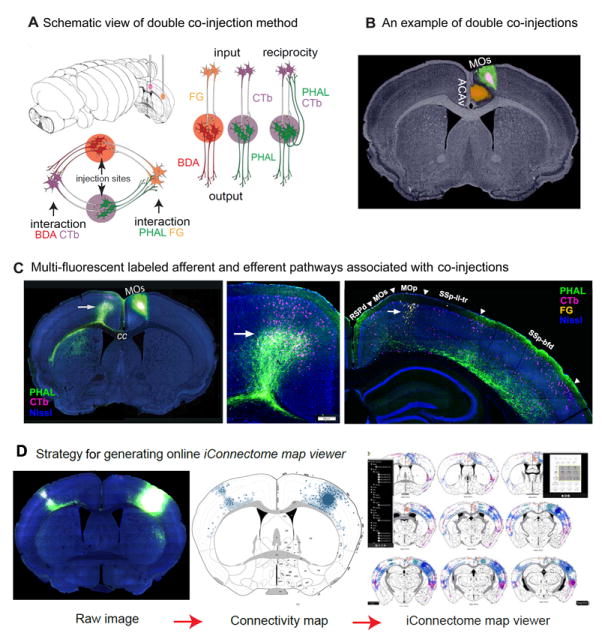
A. Schematic illustrating a PHAL/CTb and BDA/FG double co-injection in two different structures labeling both input to, and output from each injection site. Reciprocal interactions between brain regions and circuit interactions between each injection site may also be revealed. B. A coronal section showing co-injections made into the MOs and ACAv viewed with Nissl background to reveal cytoarchitecture. Scale bar: 1 mm. C. Intermixed anterogradely labeled axons (green, PHAL) and retrogradely labeled neurons (pink, CTb) in the MOs following a co-injection in the contralateral hemisphere (first two panels, arrows). Note: the PHAL/CTb co-injection is the same as pictured in B. Image histogram was adjusted differently for the two hemispheres so that PHAL/CTb labeling on the left side can be viewed properly without over exposing the injection site on the right side. Last panel, comparison of retrogradely labeled neurons from injection in ACAv (arrow, yellow, Fluorogold (FG)) and fibers and cells from injection in MOs (PHAL/CTb). Fluorescent Nissl in blue, scale bar 200μm. D. Strategy for mapping fluorescent labeling from a raw image (left, scale bar: 1mm) onto the corresponding level of the ARA (middle) to generate a comprehensive map of projection pathways for all injection sites (right). Note: anterogradely labeled pathways were rendered as layer and regional-specific shading, while retrogradely labeled neurons were represented by individual dots. The large circle on the right hemisphere represents an injection site (see corresponding region on raw image). See Figures S1, S2, S4, and Table S1 for more information.
The size of co-injections are ~ 250-500μm and mostly confined within individual cortical areas (Figure 1B), although when images are adjusted to reveal fine fibers, injection sites are overexposed, misrepresenting their actual size (Figure S1A). The confinement of the injections can be verified from the cytoarchitectural background provided by a Nissl stain of the same section (Figures 1B, S1B) and by observing their unique thalamic labeling (Figure S1A-B). The specificity of injections are cross-validated by the application of retrograde tracers to regions targeted by anterogradely labeled axon terminals and vice versa (Figure S1 for details on data validation). All images were processed through informatics pipelines and presented on the MCP website through an interactive visualization tool, the iConnectome (www.MouseConnectome.org; Figure S2A). The fluorescent connectivity data are presented in 4 different channels: PHAL (green), BDA (red), FG (yellow), and CTb (pink). Two additional channels aid in data analysis: the inverted fluorescent Nissl of the same section and the corresponding atlas level from a standard mouse atlas, the Allen Reference Atlas (ARA; Dong, 2007). Currently, a total of ~600 pathways (304 efferent and 296 afferent) associated with ~317 co-injections are available (Figure S3 for injections; Table S1 for list of selected cases, Table S2 for abbreviations). Injections span the entire neocortex and selected regions of the entorhinal cortex, hippocampus, amygdala, and olfactory areas. Although this report focuses on intracortical pathways, the subcortical connections of all injections also are available.
Connectivity matrices
To begin building cortical networks, data within all regions was annotated by manually recording the distribution of anterograde and retrograde labeling. Using the annotation data, two label-based weighted directional connectivity matrices were created (Figure 2A-D). Iterating through each matrix entry, 89% of connections exhibited mutual labeling by both anterograde and retrograde labeling methods, suggesting that the datasets were significantly similar. To reveal subnetworks, a composite matrix was constructed in which the nodes (ROIs) were reordered via a clustering algorithm (Figure 2E; Supplemental Materials for annotation and analysis details). The clustering orders nodes into modules that maximize the connectivity and arrange highly interconnected nodes such that they are clustered along the matrix diagonal, facilitating visualization of grouped regions that can be considered subnetworks. The number of connections within these groupings near the diagonal reflects the density of intraconnectivity within a subnetwork, while connections farther from the diagonal demonstrate a subnetwork’s interconnectivity with other subnetworks. The clustering demonstrated that all nodes fall into a few relatively distinct cortico-cortical subnetwork modules (Figure 2C-E). Each of the four somatic sensorimotor modules (orofaciopharyngeal, upper limb, lower limb/trunk, and whisker) formed distinct subnetworks. The medial, visual, and auditory modules formed one big network that was also highly connected with the lower limb/trunk and whisker subnetworks. The insular and temporal areas along the lateral aspect of the cortex formed two distinct clusters and the broad and unique intracortical connections of the claustrum and lateral entorhinal area suggest they may serve as hubs, or regions of high network interaction (Sporns, 2010).
Figure 2. Weighted and directed cortico-cortical connectivity matrices.
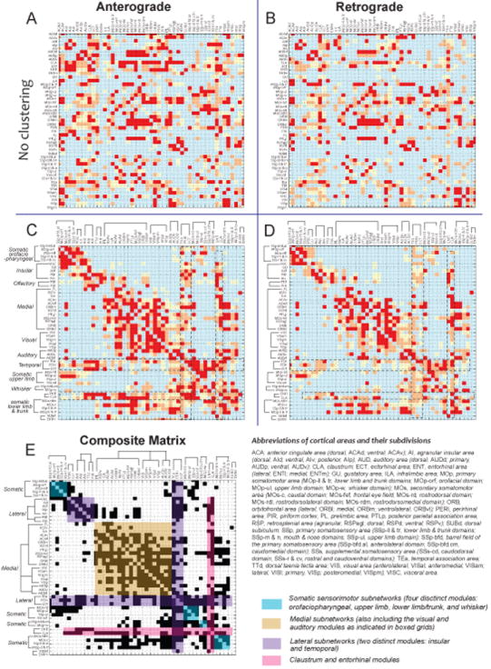
Connectivity matrices were constructed based on either anterograde (PHAL, A) or retrograde (FG/CTb, B) tract tracing data. In both matrices, connection origin is listed along the row while targets are listed across the columns (sorted alphabetically). The weighting of each connection is indicated by red (strong), orange (moderate), and yellow (light) coloring. In C and D, the anatomical data in A and B has been re-ordered illustrating a total of 12 distinct modules in different cortical subnetworks. Combining retrograde and anterograde tracing methods formed the composite matrix (E), a consensus perspective of cortico-cortical subnetwork connectivity. See Supplemental Experimental Procedures for details regarding construction of the matrices, Figure S3 for injection cases, and Table S2 for list of abbreviations.
Cortico-cortical connectivity map
The matrices provide a condensed view of cortical connectivity patterns, but exclude details like projections routes, laminar specificity of projections, or topographical and topological connectivity patterns, which are critical features of networks. Consequently, labeled pathways were manually reconstructed onto corresponding atlas levels to create a comprehensive cortico-cortical connectivity map available through the iConnectome map viewer (Figures 1D, S2B, S4A; http://www.MouseConnectome.org/CorticalMap/).
This map includes 80 anterograde (PHAL) and 160 retrograde pathways (CTb and FG). The co-injection sites are represented by circles, PHAL pathways by shaded regions, and retrograde labeling by small dots that reflect regional and laminar distribution patterns (Figures 1D, S4A). Each of these pathways was assigned a unique RGB value and rendered into an individually layered document such that multiple layers representing multiple injection sites could be viewed simultaneously within the same anatomic frame (ARA), thus revealing topographic trends and interactions between regions. Within the connectivity map, when nodes within the same module of the connectivity matrix are viewed together (e.g., anteromedial and anterolateral visual areas), intermixed and overlapping cortical connectivity patterns are observed suggesting a high degree of integration within the same subnetwork (Figure S4B-C). Conversely, nodes of different modules show divergent cortical connections.
The somatic sensorimotor subnetworks
To build the somatic sensorimotor subnetworks, four general primary somatosensory (SSp) domains were defined based on their sub-cortical and intracortical connections (Figure 3A-B): the mouth and nose (SSp-m/n), upper limb (SSp-ul), lower limb and trunk (SSp-ll/tr), and barrel field (SSp-bfd). The specificities of these domains were validated by examining their specific somatotopic projections in sensory and motor related nuclei in the lower brainstem (Figure S5A-B). Each of these SSp domains displays unique connectional patterns with other somatic sensorimotor areas like the primary (MOp) and secondary (MOs) motor areas, and the secondary somatosensory cortex (SSs) (Figures 3A-B, S5C). These distinct connections provided a structural basis for delineating related sub-domains within each of these motor areas, which are largely unknown in the mouse. Parcellations were confirmed by the application of co-injections into the corresponding body subfield domains of the somatic sensorimotor cortical areas (i.e. SSp-ll/tr, MOp-ll/tr, MOs-ll/tr; Figure 3C).
Figure 3. The somatic sensorimotor subnetworks.
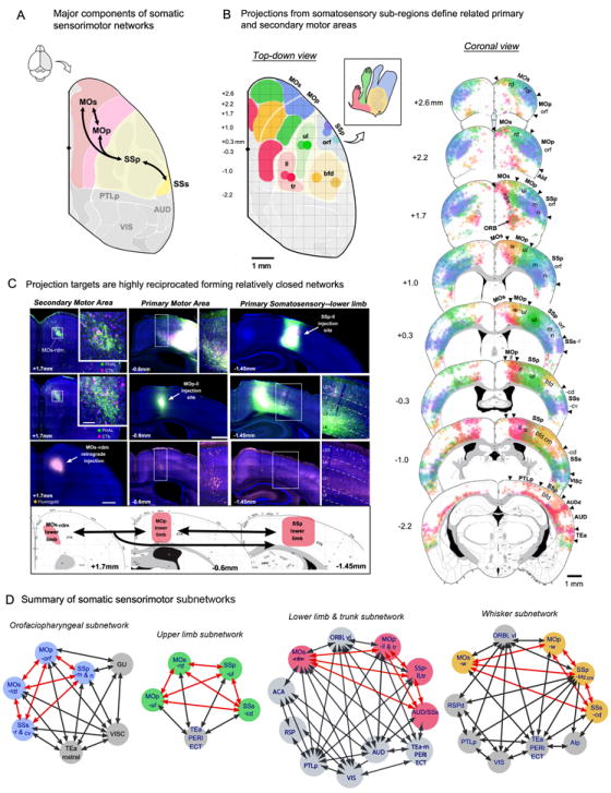
A. Overview of the four major components of somatic sensorimotor areas (SSp, SSs, MOp, MOs). Each region is extensively interconnected with all others. Parcellation of cortical areas in map based on ARA and drawn to scale. Diamond shape on midline indicates bregma. B. Projections from representative injection sites (colored dots) in each of four basic body representations in primary somatosensory cortex: orofaciopharyngeal (orf, blue), upper limb (ul, green), lower limb and trunk (ll/tr, red), and whisker-related caudomedial barrel field (bfd.cm, yellow). A cartoon (inset) shows approximate size and location of the four body areas defined here (inspired from Brecht et al. 2004). Top-down view (left) shows topographic organization of projections from each area to corresponding primary and secondary motor areas (MOp, MOs). ARA defined boundary between MOs and MOp added for reference. Projection data in top-down view were drawn to scale using coronal sections (right) and shaded regions represent the areal extent of the most dense projections from each of the injected regions. Representative coronal sections also show projection trends to supplemental somatosensory area (SSs). Numbers indicate position of sections relative to bregma (mm). C. Projections from each of the somatosensory sub-regions define presumably functionally related MOs and MOp sub-regions, which are tightly reciprocated, as indicated by closely overlapped axonal fibers and retrogradely labeled cell bodies following co-injection. Here, co-injections of PHAL (green)/CTb (pink) in either SSp-ll (top panel, right) or a corresponding MOp region (middle panel, middle) reveal intermixed labeling in other corresponding domains of the somatic sensorimotor region, confirming their strong reciprocal connectivity. Both co-injections reveal intermixed labeling in the same MOs domain (left images on the top and middle panels). Retrograde injection in the same MOs domain (left image on the lower panel) confirms the specificity of this interaction, showing retrogradely labeled neurons in the former two areas (middle and right images). Their anatomical locations and interactions are summarized in corresponding atlas levels in the bottom panel. Scale bars 500μm and 100μm (inset). D. Building on these observations, four network graphs were created using each of the defined somatosensory regions as starting points. Each subnetwork is distinct and all components within it share a high degree of interconnection. Each are composed of several somatic sensorimotor “nodes” (color coded to match anatomically defined functional domains in B) that are reciprocally connected (as indicated with red arrows). Each of these subnetworks also includes other non-somatic “peripheral” nodes (gray circles) and their connections are shown with gray arrows. See also Figure S5. For abbreviations of nomenclatures, please see Figure 2 and Table S2.
These somatic sensorimotor areas formed four distinct subnetworks. The orofaciopharyngeal subnetwork is composed of five major nodes (Figures 2, 3B): (1) SSp-m/n; (2) the orofacial region of the MOp (MOp-orf; Yamada et al., 2005); (3) the rostrodorsolateral MOs (MOs-rdl); (4) anterolateral SSp-bfd (SSp-bfd.al); and (5) the rostral and caudoventral SSs (SSs-r & cv). Co-injections into each of these orofaciopharyngeal nodes showed they are all heavily reciprocally interconnected (Figure 3D). The gustatory (GU), visceral (VISC), and dorsal agranular (AId) areas also connect with this subnetwork (Figures 2, 3D), which could contribute relevant information (i.e. gustation and food safety; Carleton et al., 2010; Maffei et al., 2012).
Following the same topological organization (i.e. reciprocity among all nodes), the upper limb subnetwork is composed of four somatic sensorimotor nodes: (1) the SSp-ul; (2) caudodorsal SSs caudodorsal (SSs-cd); (3) MOp-ul; and (4) rostrodorsal MOs (MOs-rd) (Figures 3D, S5B). The lower limb/trunk subnetwork includes the SSp-ll/tr, MOp-ll/tr, and rostrodorsomedial MOs (MOs-rdm) (Figure 3B-D). Finally, the whisker subnetwork is composed of the caudomedial SSp-bfd (SSp-bfd.cm), MOp-w, which corresponds to the vibrissal primary motor cortex (vM1) (Mao et al., 2011; Gerdjikov et al., 2013), and the caudodorsal SSs (SSs-cd; Figure 3B,D). The upper limb, lower limb/trunk, and whisker subnetworks also share connections with lateral subnetwork nodes like the temporal association (TEa), perirhinal (PERI), and ectorhinal (ECT) areas. Relevant information for the lower limb/trunk subnetwork also may be provided by inputs from the visual (VIS), auditory (AUD), and several areas within the medial networks (Figures 2, 3D).
Finally, a specific frontal eye field MOs domain (MOs-fef, Figure S5D; Reep et al., 1990) was identified, which shares dense reciprocal connections with the visual, auditory, posterior parietal, anterior cingulate, and restrosplenial areas of the medial subnetworks.
The medial subnetworks
Cortical areas along the medial bank of the cortex cluster to form two parallel medial subnetworks (Figures 2, 4A). The first medial subnetwork is organized for transferring visual, auditory, and somatic sensory information to the ORBvl. ORBvl co-injections showed its direct reciprocal connections with the primary (VISp) and secondary visual (anteromedial, VISam; anterolateral, VISal) and auditory areas (AUD), as well as the SSp-ll/tr and SSp-bfd.cm (Figures 2, 4A-C). Co-injections into each of these areas confirmed these connections (Figure S4B-C for VISam and VISal; Figure S6A for VISp and AUD; Figure 3B for SSp-ll/tr). Further, multiple retrograde tracers injected into different visual areas revealed dense ORBvl neuronal labeling that was intermixed, but mostly not co-localized suggesting multiple parallel ORBvl→VIS pathways (Figure 4E-F).
Figure 4. The medial subnetworks.

A. Major components of the medial subnetworks, which mediate transduction of information between sensory areas (VIS, AUD, and caudal-most SSp) and higher order association areas along the medial bank of the neocortex, such as the retrosplenial (RSP), parietal (PTLp), anterior cingulate (ACA), and orbital (ORB) areas. B. Connectivity pathways of the medial subnetwork revealed by co-injections in the ORB (note: these are aggregated pathways for three different cases, see three co-injection sites in ORB, colored pink, light brown, and dark brown, medial to lateral). C. Representative raw images from an ORBvl co-injection. PHAL labeled axons and CTb labeled neurons are found in other medial network components such as the ACAd and adjacent MOs-fef, PTLp, RSPd, and primary and secondary VIS areas (VISp, VISal and VISam). Scale bars 500μm (first panel) and 200μm. D. Laminar specific differences in axonal projections to primary visual cortex (VISp) arising from either ORBvl (red, BDA labeling) or ACAd (green, PHAL). Injection sites in the same brain, left panels, scale bars 500μm (left) and 1mm. Projections to different layers of the same section of VISp (right panels). Underlying fluorescent Nissl was inverted to aid visualization of layers (right-most panel). Scale bar 200μm. E. Four different retrograde tracers were injected into the VISp (two), VISam, and VISpm within the same brain, resulting in distinct, topographically arranged clusters of neurons in the ACA and adjacent MOs-fef. In the ORBvl, these retrogradely labeled neurons are intermixed, but mostly not colocalized (bottom right, 5% colocalization for any combination of tracers in ORBvl, 436 cells counted, 21 had two or more tracers present). Scale bars: 1mm (top left), 500μm (bottom left), 200μm (top right), 100μm (bottom right). F. Summary of interactions among the medial subnetworks. Left, interaction between sensory and association areas. Dashed lines indicate sparse connection. Claustrum (CLA) is included due to high degree of interconnection with medial network. Middle, connections between the association areas. Thicker arrows indicate dense projection patterns between regions. Dashed line separates a direct pathway to medial prefrontal region along the ventro-medial bank of the cortex (second medial subnetwork). Asterisks indicate a unidirectional connection between CLA and RSP. Right panel, overview of medial network interactions including TEa and parahippocampal structures (i.e. SUBd, ENTm), which project to RSP (red arrows). Reciprocal connections of visual (blue) and auditory (green) areas with all major medial network components shown. Caudal-most somatosensory areas (SSp-ll/tr; SSp-bfd.cm) are included as well (gray arrows). See also Figure S6.
These VIS and AUD areas also reciprocally connect with areas along the cortical medial bank, including the posterior parietal (PTLp), three subdivisions of the retrosplenial area (dorsal, RSPd; agranular, RSPagl, and ventral, RSPv), and two subdivisions of the anterior cingulate area (dorsal; ACAd; ventral, ACAv) (Figures 2, 4A-C, 4F, S6A-B). The PTLp is another critical area that integrates inputs from the VIS, AUD, and SSp-ll/tr (Figures 2, 3B, S6A). The RSPd and RSPagl receive much stronger visual inputs, but only sparse AUD and SSp projections (Figures 2,S6A). In the ACA, axons from different VIS and AUD areas intermix in layer 1 (Figure S6A), while neurons that project to the VISp and VISam form different clusters in deeper layers (Figure 4E).
Moreover, the ORBvl and all of these higher order association areas (PTLp, RSP, ACA) heavily interconnect with regional and laminar specificity (Figures 4A-C,F, S6B). For example, in the PTLp, the densest labeling from ORB injections are distributed in layer 5 (Figure 4B-C); ACAd axons are distributed primarily in PTLp layers 1 and 6 and retrogradely labeled neurons across layers 2 to 6 (Figure S6B). Projections from these areas to lower order sensory areas also are laminar specific with ORBvl axons primarily distributing in layers 1 and 5 of visual areas, while ACAd axons reside in layers 1 and 6 (Figures 4C-D, S6B).
Interestingly, this medial subnetwork provides an interface for direct interactions between different sensory modalities via reciprocal connections among the visual and auditory areas and the SSp-ll/tr and SSp-bfd.cm (Figures 2, 3B, S6C-D). This supports the concept of cross-modal modulation, which challenges the idea that mammalian primary sensory cortices are strictly unisensory (Driver and Noesselt, 2008; Stein and Stanford, 2008). Finally, this medial network may be important for translating sensory information into motor action since the ORBvl, ACAd, and PTLp connect with the entire MOs including the MOs-fef and the ORBvl and PTLp further connect with the MOp-ll/tr (Figures 4B-C,F, S5D).
The second medial subnetwork successively relays information from the dorsal subiculum (SUBd) to the medial prefrontal cortex (Figure S6E). The RSPv is the only neocortical recipient of dense inputs from the SUBd, through which information processed in the dorsal hippocampus can reach the neocortex (Fanselow and Dong, 2010). The RSPv shares massive reciprocal connections with the ACAv. It in turn projects to medial prefrontal cortical areas like the infralimbic (ILA), prelimbic (PL), and medial orbitofrontal areas (ORBm) (Figure S6E), each of which receive only sparse inputs from the RSPv (Figure 4F).
Importantly, the two medial networks can interact (Figure 4F) since the RSPv and ACAv are connected with the ORBvl, ACAd, RSPd, RSPagl, and PTLp. Finally, these medial subnetwork areas are all connected with the CLA (Figures 2, 4B,F, S6B)
Lateral subnetworks
Cortical areas in the lateral aspect of the neocortex form two distinctive, highly interconnected networks (Figures 2, 5A): the anterolateral insular and posterolateral temporal subnetworks. Distinguishing the lateral networks from the medial and somatic sensorimotor subnetworks is the fact that the lateral subnetworks share connections with olfactory cortical areas (piriform cortex, endopiriform nucleus, dorsal taenia tecta), basolateral amygdalar nucleus, and ventral hippocampus.
Figure 5. The lateral subnetworks.

A. Sagittal view of the major components of two lateral subnetworks: the anterolateral insular (including the AId, AIv, AIp, VISC, GU) and posterior temporal (including TEa, ECT, PERI). These two interconnected subnetworks are also connected with olfactory (e.g. PIR) and medial prefrontal (mPFC) areas and with the ENTl. TEa in particular forms extensive connections with much of the rest of the neocortex (gray arrows). B. Distinct projection patterns of the anterior agranular areas (PHAL injections involved both AId and AIv, left panel) and AIp (right panel) with the mPFC areas (PL, ILA, DP), posterior temporal areas (TEa, ECT, PERI), and ENTl. The AIp targets more ventral structures in mPFC and more heavily innervates the central nucleus of the amygdala (CEA). Scale bars: 500μm. C. Map of neuronal inputs to (left panel) and output from (right panel) the TEa, which are arranged topographically along the rostrocaudal direction. Note: these pathways are aggregated from 6 co-injections made into different parts of the TEa from rostral (red) to caudal (blue) direction (top most sagittal image, numbers relative to bregma in mm). Retrogradely labeled neurons are indicated as colored dots and demonstrate the layer specific origin of cortical projections to TEa. Axonal pathways arising from TEa (outputs) are rendered as shaded areas of color. D. Raw image of retrograde labeling (FG, yellow) following injection in TEa. Cells are distributed extensively across numerous cortical regions following a single, small injection, suggesting a high level of convergence. Bottom left panel shows close up of layer specificity in somatosensory barrel field, with most cell bodies residing in upper layer 2/3, 5a, and some layer 6. Fluorescent Nissl inverted (right) to aid in discriminating layers. Layer 4 “barrels” indicated with arrow. Scale bars: 500μm(top) and 200μm (bottom). E. Raw image of co-injection in TEa. Fibers are predominately ipsilateral, but retrogradely labeled inputs are evenly distributed across both hemispheres. See right panel, middle, comparing labeling in contralateral and ipsilateral MOs. Scale bars: 1mm (top right), 200μm (middle), 500μm (bottom). See also Figure S7.
The anterolateral insular subnetwork is composed of the three agranular insular areas: the dorsal (AId), ventral (AIv), and posterior (AIp). The neural connections of the rat AI have been investigated (e.g., Saper, 1982; Allen et al., 1991; Jasmin et al., 2004), but their functional and structural differences remains controversial. Our data show that these subdivisions are substantially interconnected, but generate distinguishable cortical projections (Figure 2). First, connections between these three areas and the medial prefrontal cortex display a rough topography (Figures 5B, S1E): the AIp is heavily connected with the poorly defined dorsal peduncular area (DP) (all layers) and its dorsally adjacent ILA (layers 1 and 6), but relatively sparsely with the PL. The AIv has the densest reciprocal connections with the PL, ILA, and DP. The AId is interconnected with the PL, but sparsely with the ILA and not at all with the DP. An ILA co-injection validated this preferential interaction between AIv and ILA (Figure S1E). Second, all three AI areas connect with the VISC, but only AId and AIp are significantly connected with the GU. The VISC receives visceral inputs from the parvicellular part of the ventral posterolateral thalamic nucleus (VPLpc), while the GU shares massive reciprocal connections with the parvicellular part of the ventral posteromedial thalamic nucleus (VPMpc; Figure S1B) (Jones, 2000). Third, the AId also is connected with the orofaciopharyngeal (MOp-orf and MOs-rdl) and upper limb (MOs-rd) subnetworks, while the AIp receives significant inputs from the SSs and SSp-bfd (Figure S7A).
Caudally, these AI subdivisions preferentially connect with three components of the posterolateral temporal subnetwork (Figure 5B): the perirhinal (PERI) receives dense inputs from the AId and AIv, while the ectorihinal (ECT) is more heavily innervated by inputs from the AIp. Finally, all three generate dense inputs specifically to layers 3-5 of the lateral entorhinal cortex (ENTl; Figures 5B; S1B).
Three areas located in the vicinity of the rhinal fissure, namely the temporal association area (TEa), ECT, and PERI form the highly interconnected posterolateral temporal_subnetwork (Figures 2, 5A,C). A retrograde tracer injection in all three structures back labeled neurons in layers 2 and 5a of the entire neocortex with the exception of the ACAv, RSP, and VISp (Figure 5C-D) suggesting that this subnetwork receives input from nearly the entire neocortex. Complementarily, the TEa, ECT, and PERI collectively project back to nearly the entire neocortical mantle including the VISp (Figure 5C,E).
Injections in all other cortical areas revealed heterogeneous zones within the TEa (Figure S7B). The rostral TEa shares bidirectional connections with areas in the orofaciopharyngeal network; the middle TEa and its adjacent PERI and ECT share stronger connectivity with somatic sensorimotor areas of the upper limb and lower limb/trunk subnetworks, visual and auditory areas, as well as the PTLp; the caudal TEa more specifically connects with the medial prefrontal areas and ventral hippocampus.
Finally, co-injections in the TEa, PERI, ECT result in dense labeling in layers 3-5 of the ENTl (Figure 5C).
ENTl and CLA subnetworks
The ENTl and CLA are two reciprocally connected structures that both share connections with the medial prefrontal (ILA, PL, ORBm) and orbitofrontal areas (ORBvl, ORBl) (Figures 2, 6A,E,G). The CLA further shares massive connections with cortical areas within the medial (ACAv, ACAd, PTLp, RSPd, RSPagl) and lateral subnetworks (AId, AIv, AIp, TEa, PERI, ECT), as well as with the entire MOs and MOp (Figure 6A-D). Dense CLA axons travel through layers 5 and 6 of all sensory areas (SSp, AUD, VIS), although these cortical areas contain relatively few neurons that project back to the CLA. The intracortical connectivity of the CLA displays a unique asymmetric pattern: cortical inputs to the CLA are bilateral, but outputs from CLA are almost exclusively ipsilateral (Figure 6B-C).
Figure 6. The CLA and ENTl.
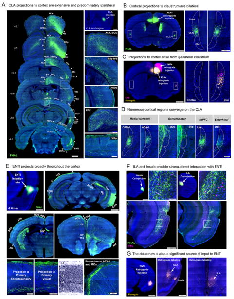
A. Axonal projections arising from the CLA are distributed throughout the entire neocortex and ENTl on the ipsilateral hemisphere. Note: these axons display different regional and laminar distribution specificity (on right panel) Scale bars: 1mm (left), 500μm (top right), 200μm (bottom). Panels B and C show asymmetric connections of the CLA with other cortical areas in the two hemispheres. Cortical inputs to CLA project to both sides with equal densities (B, labels: dorsal and ventral claustrum (CLAd, CLAv), and endopiriform nucleus (EPd)), while outputs from CLA to other cortical areas indicated by retrograde tracers are almost exclusively ipsilateral (C). Moreover, the CLA has a dorsal to ventral topography in its projections to the cortex, with cells in CLAv (yellow, C, right panel) preferentially targeting ventral cingulate (C, left panel, injection site in ACAv). Very little co-labeling was observed among cells labeled from a neighboring, more dorsal injection (pink). Scale bars: 1mm (left) and 200μm (right). D. Neural inputs to the CLA from almost all cortical areas in medial, somatic, and lateral subnetworks. The somatomotor inputs preferentially target the dorsal-most aspect of CLA. E. Representative images of PHAL labeled axons in layer 1 of a wide range of neocortical areas arising from the rostrodorsal ENTl. F. Laminar specificity of PHAL labeled axons and CTb labeled neurons in the ENTl after co-injections made into the AI or ILA. Both cortical regions provide strong, direct input to ENTl, further supported by retrograde data in G. These data also confirm the CLA is a specific source of input to ENTl (G, middle panel). Scale bars: 1mm (F, top left and G, left), 500μm (F, bottom and G, middle), 100μm (F, top right). See also Figure S1B-E.
The ENTl shares much stronger reciprocal connections with all areas of the lateral subnetworks (Figures 5A-C, 6F), amygdala (basomedial and anterior basolateral nuclei), and the ventral and intermediate CA1 and SUBd (data not shown). The ENTl receives direct inputs from the main olfactory bulb (Hintiryan et al., 2012) and shares massive reciprocal connections with olfactory cortical areas like the piriform and taenia tecta (Figure 6E). These data suggest that the ENTl is not only a gateway for neocortical information to the hippocampus (de Curtis and Paré, 2004), but may also be a site of interaction for various cortical areas and between these neocortical areas and the amygdala, hippocampus, and olfactory cortical areas.
Compared to the CLA, the ENTl receives very sparse or no direct inputs from regions within the medial subnetworks (ACA, RSP, PTLp) and somatic sensorimotor subnetworks; however, co-injections into layers 4/5 of the rostrodorsal ENTl revealed dense axons throughout layer 1 of almost the entire neocortex (Figure 6E) with a few exceptions—the RSPv and areas within the orofaciopharyngeal subnetwork. Notably, the ENTl layer 1 axons are denser in the contralateral visual, auditory, and SSp-bfd areas.
Interactions with the prefrontal cortex
Projections from each of the identified subnetworks topographically converge onto discrete regions of the prefrontal cortex. The somatic sensorimotor subnetworks primarily converge onto the dorsolateral, dorsal, and dorsomedial sectors of the rostral-most MOs (Figures 3B, 7A-B). Together, these three neighboring zones occupy the dorsolateral half of the prefrontal cortex (PFCdl, Figure 7A-B).
Figure 7. Interactions with prefrontal cortex.

Cumulative projections from components of the somatic sensorimotor, lateral, and medial networks in two representative coronal sections of the prefrontal cortex (PFC) (A-B). Collectively these represent inputs from the entire neocortex to the PFC. Inputs were color coded based on the location of the injection sites in different components of the network (A). For example all primary motor projections arising from multiple injections along the length of this structure were colored green and all somatosensory projections were colored blue (A, top). ACAv was colored red to separate it as a component of the second medial subnetwork (A, bottom, see Fig S6E). Note that RSP has very little interaction with the PFC. B. All inputs from three somatic sensorimotor subnetworks (as shown in A) converge onto three distinct zones, dorsolateral (dl), dorsal (d), and dorsal medial (dm), in the dorsolateral half of the prefrontal cortex (PFCdl, green and blue). In contrast, the medial and lateral subnetworks converge onto the ventromedial half of the prefrontal cortex with distinctive patterns. Note that caudal-most somatosensory and motor regions make some contribution to lateral-most, and caudal aspects of ORB (green and blue shading). C. A schematic view of cortico-cortical network information flow as seen in a top-down view of the cortex (left, lateral edge on left, PFC at the top). All subnetworks are colored according to the scheme used in A and B. Right, a more detailed overview of these interactions (lateral edge of cortex on the right, PFC at the top). Somatic sensorimotor boxes are meant to include both the sensory area and its corresponding primary motor area with which it is strongly interconnected. All functionally distinctive subnetworks are organized along the longitudinal axis of the cerebrum. Information processed in the medial and lateral subnetworks is integrated within the ventromedial half of the prefrontal cortex (PFCvm) and the ENTl. The claustrum (CLA) may also provide an additional means of direct interaction between each of the subnetworks. For abbreviations, please see Figure 2 and Table S2. Additional abbreviations: AMY, amygdala; AH, Ammon’s Horn; HPF, hippocampal formation.
The ventromedial half of the prefrontal cortex (PFCvm) is also composed of three distinct zones: the medial prefrontal (ILA, PL, ACAd, ORBm), orbitofrontal (ORBvl, ORBl), and the anterior-most part of the agranular insular areas (AId, AIv). The medial prefrontal zone reciprocally connects with the AI and caudal TEa of the lateral subnetworks potentially acting as a site for medial and lateral subnetwork integration. This information arrives at the medial prefrontal zone via two routes (Figure 7A). The dorsal route links the dorsomedial corner of the prefrontal cortex (PL, ACAd) with the ventrolaterally located AId. The axons through this route make a 45° cut that demarcates the border between the dorsolateral and ventromedial halves of the prefrontal cortex. The ventral route links the medial (ILA) and lateral (AIv) areas across the orbitofrontal areas.
Overall, most components of the medial subnetwork communicate with the orbitofrontal zone. The ORBvl and ORBl are targets of projections from the VIS, AUD, and PTLp. The orbitofrontal zone also receives input from the TEa (lateral subnetwork) suggesting that, like the medial prefrontal cortex, it may also serve as a site of integration for the medial and lateral subnetworks.
Aside from the strong interaction between the medial prefrontal and insular zones, very little interaction is observed among the other neighboring structures of the prefrontal cortex. For example, co-injections in the ORBvl show no projections to or from the PFCdl and medial prefrontal areas. The relative segregation of these prefrontal zones combined with their specific cortical inputs and subcortical targets may help define their unique processing role and contribution to behavior.
DISCUSSION
The iConnectome: an open resource of multi-format connectivity data
Open resources providing access to neurohistological images are revolutionizing neuroanatomy (Jones et al., 2011). The iConnectome is an online resource that presents high-resolution whole-brain images of neural connectivity in several different formats. Imaging data are presented in which labeled axonal pathways and neurons can be viewed with their own Nissl background or their corresponding anatomic ARA map. Cortico-cortical connectivity matrices (Figure 2) provide an overview of inter-cortical connections. Cortical connectivity matrices that comprise virtually all of the neocortex have been generated in different species using data available in the literature (Honey et al., 2007; Sporns et al., 2007; Markov et al., 2010; for rat see BAMS: http://brancusi.usc.edu/). In contrast, the networks reported here are based on data collected and analyzed in a homogenous fashion rather than gathered piecemeal from the literature. The cortical connectivity map allows users to directly compare connectivity patterns of different cortical areas within the same neuroanatomic framework. Taken together, these resources allow researchers to conceptualize any cortical region of interest in the context of larger network interactions.
The cortical subnetworks
Examination of the full data set revealed that the neocortex is organized into several subnetworks that display unique topological organization, perhaps reflecting different information processing strategies for each. Within the somatic sensorimotor network, all main somatic nodes within the four subnetworks are heavily and reciprocally connected. This organization allows direct interactions between sensory and motor areas in the absence of higher order association areas. This pattern could enable rapid integration of different sensory modalities for dynamically regulating motor actions, such as the integration of tactile information in the oral cavity and proprioception of the jaw for initiation, maintenance, or termination of rhythmic jaw movements throughout the masticatory period (Tsumori et al., 2012; Yamada et al., 2005).
Unlike direct sensorimotor interactions that occur within the somatic sensorimotor subnetworks, the first medial subnetwork primarily mediates interactions between the sensory and higher order association areas. The first medial subnetwork serves to transmit sensory information from the visual, auditory, and somatic sensory (SSp-ll /tr and SSp-bfd.cm) areas to the ORBvl and is organized differently than the sensorimotor subnetworks. All of the sensory areas directly connect with the ORBvl through multiple parallel pathways. Each of these areas is also connected with higher order association areas like the RSPd, RSPagl, RSPv, PTLp, ACAd, and ACAv, within which sensory inputs can be integrated prior to reaching the ORBvl. Almost all cortical areas in this network (ORBvl, ACA, RSP, PTLp) have been implicated in orientating and coordinating movements of the eyes, head, and body in object searching tasks and spatial navigation (Feierstein et al., 2006; Bucci, 2009; Vann et al., 2009; Weible, 2013).
The second medial subnetwork is topologically distinct from the first in that it successively transmits information from the SUBd to the RSPv to the ACAv and then to the ILA, PL, and ORBm. This multi-synaptic subnetwork may provide a structural basis for relaying information processed in the dorsal hippocampus and SUBd, perhaps regarding spatial orientation, navigation, and episodic memory, to the medial prefrontal cortex (Vann et al., 2009; Fanselow and Dong, 2010; Weible, 2013).
The lateral subnetworks represent a point of massive convergence in the cortex. Interactions are centered on two major components: the AI in the anterolateral insula subnetwork, and the TEa/PERI/ECT complex in the posterolateral temporal subnetwork. Each receives input from, and projects back to, an extensive number of cortical areas. For example, the anterolateral insular subnetwork integrates gustatory, visceral, and olfactory information, while the posterolateral temporal subnetwork processes more visual, auditory, somatosensory, and motor information. Both subnetworks then transfer this information rostrally to the medial prefrontal cortex and caudally to the ENTl. These connectivity patterns may support the proposed role of the AI in self-awareness of internal states (Craig, 2009) and the role of the TEa/PERI/ECT in perception, object recognition, and contextual memory associated with emotion (Winters et al., 2008; Aggleton et al., 2010).
Interactions among the subnetworks
Importantly, several regions of the cortex potentially serve as sites for subnetwork interaction. The PFCdl receives a confluence of information from all four somatic sensorimotor subnetworks. The PFCvm receives convergent inputs from the medial and lateral subnetworks and provides an interface for integrating or communicating information regarding external stimuli (such as visual, auditory, somatic sensory) and internal stimuli (such as visceral and gustatory information). The CLA provides another means by which the medial, lateral, and even the somatic sensory subnetworks may directly interact. Both the PFCvm and CLA are directly interconnected with the ENTl, which further receives massive, highly integrated sensory information from the two lateral subnetworks. Through the ENTl, this information may reach the hippocampus, amygdala, and olfactory cortical areas, or be routed directly back to the medial prefrontal cortex (Figure 7C). In addition, the ENTl is also the starting point of the classic trisynaptic circuit that transfers information to the hippocampus, which may ultimately reach one of its main output targets, the SUBd (Witter, 2007) to re-enter the medial network through its projections to RSPv. Consequently, through the prefrontal cortex, ENTl, and CLA, information has the potential to be represented and communicated throughout the limbic loop surrounding the entire neocortex (Figure 7C).
Conclusion and perspective
In conclusion, we and other groups have demonstrated the feasibility of producing and collecting large-scale connectivity data (Osten and Margrie, 2013; Pollock et al., 2014); however, interpretation of this wealth of anatomical data presents an ongoing challenge. This resource provides a reference for determining the complete set of inputs and outputs for a given cortical region and for implicating it in a broader network context. Any of these long range interactions may be validated at the synaptic level using transsynaptic viral tracing and may be further investigated to determine cell-type specific connections using methods such as channelrhodopsin-assisted circuit mapping (Luo et al., 2008; Osakada et al., 2011; Petreanu et al., 2009). Moreover, these projections may be assessed functionally using available optogenetic techniques that allow one to measure the circuit-level or behavioral consequences of manipulating a given pathway within a neural network (Yizhar et al., 2011).
EXPERIMENTAL PROCEDURES
Data generation, collection, and online presentation
All experimental procedures have been described previously (Hintiryan et al., 2012). In brief, double co-injections of tracers were made into different areas of the entire neocortex, hippocampus, olfactory cortical areas, and amygdala of 8 week old male C57Bl/6J mice. PHAL (2.5%; Vector Laboratories) and CTb (647 conjugate, 0.25%; Invitrogen) were co-injected, while BDA (FluoroRuby, 5%; Invitrogen) was injected in combination with FG (1%; Fluorochrome, LLC). One week was allowed for tracer transport after which animals were perfused and their brains extracted. All brains were sliced at 50μm thickness using a Compresstome (VF-700, Precisionary Instruments, Greenville, NC). One series of sections was stained for PHAL using Alexa Fluor® 488 (Invitrogen). All sections were counterstained with a fluorescent Nissl stain, NeuroTrace® 435/455 (NT; 1:1000; Invitrogen). The sections were then mounted, coverslipped and scanned as high-resolution virtual slide image (VSI) files using an Olympus VS110 high-throughput microscope. The VSI files were converted to tiff format prior to being registered. Following registration and registration refinement pipelines, the NeuroTrace® fluorescent Nissl was converted to bright-field. Next, each of the five channels for every image was adjusted for brightness and contrast to maximize labeling visibility and quality in iConnectome. Following final modifications (i.e. skewness, angles) and JPEG2000 file format conversions, images were published to iConnectome. For more details on experimental procedures, see Supplemental Materials.
Data annotation and construction of cortical connectivity matrices and connectivity map
Currently, informatics tools that automatically and precisely identify fine anatomic boundaries in histological brain sections are non-existent. Consequently, analysis of the data necessitates manual annotation to index anatomic locations and semi-quantitative strengths of labeled cortico-cortical pathways. Analysis is performed in two formats. The first is for the purpose of constructing a comprehensive connectivity database and is comprised of an excel sheet that indexes anatomic locations and corresponding semi-quantitative densities of labeling (PHAL labeled axons/terminal boutons; CTb and FG labeled neurons). These data were used to generate connectivity matrices (see Supplemental Materials). The second method consists of manually rendering the observed labeling patterns using Adobe Photoshop. Each pathway is rendered in a separate layer and all layers across all experiments are stacked to allow for a composite view of labeling trends.
Supplementary Material
Highlights.
Imaging database of mouse cortical connectivity
Interactive cortical map allowing direct comparison of cortical projection data
Identification of topologically distinct cortical subnetworks
Insights into the connectivity architecture of the mouse neocortex
Acknowledgments
The authors would like to thank Drs. Larry Swanson and Harvey Karten for advising this project, Daren Lee, Anand A. Joshi, Nikhil G. Sane, and Queenie Ng for the initial development of the iConnectome visualization tool and Betty W. Lee, Carlos Mena, Vaughan Greer, and Robert De La Cruz for their contributions to the website. We acknowledge Arleen Grewal, Annie Chen, Amy Hwang, and Hyojin Ryu for their contributions in image processing. This work was supported by NIH/NIMH, MH094360-01A1 (HWD) and P41 Supplement (AWT 3P41RR013642-12S3). This manuscript is dedicated to Dr. Edward (Ted) G. Jones, a devoted scientist, colleague, and beloved friend who will be greatly missed.
Footnotes
Author Contributions
B.Z., H.H., L.G., M.Y.S, M.B, M.S.B., N.N.F., and H.-W.D. produced, processed, and analyzed the data and prepared the images for publication into the iConnectome. B.Z. constructed the cortico-cortical connectivity map. S.Y. developed the interactive iConnectome connectivity map viewer. S.Y. also participated in the initial design of iConnectome visualization tool and the development of the informatics pipeline for data processing. I.B. and M.S.B. performed network analysis and constructed connectivity matrix. H.-W.D., H.H., and B.Z. wrote the manuscript. All authors made constructive comments on the manuscript. A.W.T. served as project advisor and participated in the planning and organizing of the project. H.-W.D. conceived and led the project.
Publisher's Disclaimer: This is a PDF file of an unedited manuscript that has been accepted for publication. As a service to our customers we are providing this early version of the manuscript. The manuscript will undergo copyediting, typesetting, and review of the resulting proof before it is published in its final citable form. Please note that during the production process errors may be discovered which could affect the content, and all legal disclaimers that apply to the journal pertain.
References
- Aggleton JP, Albasser MM, Aggleton DJ, Poirier GL, Pearce JM. Lesions of the rat perirhinal cortex spare the acquisition of a complex configural visual discrimination yet impair object recognition. Behav Neurosci. 2010;124:55–68. doi: 10.1037/a0018320. [DOI] [PMC free article] [PubMed] [Google Scholar]
- Allen GV, Saper CB, Hurley KM, Cechetto DF. Organization of visceral and limbic connections in the insular cortex of the rat. J Comp Neurol. 1991;311:1–16. doi: 10.1002/cne.903110102. [DOI] [PubMed] [Google Scholar]
- Andrews-Hanna JR, Reidler JS, Sepulcre J, Poulin R, Buckner RL. Functional-anatomic fractionation of the brain’s default network. Neuron. 2010;65:550–562. doi: 10.1016/j.neuron.2010.02.005. [DOI] [PMC free article] [PubMed] [Google Scholar]
- Behrens TE, Sporns O. Human connectomics. Curr Opin Neurobiol. 2012;22:144–53. doi: 10.1016/j.conb.2011.08.005. [DOI] [PMC free article] [PubMed] [Google Scholar]
- Bohland JW, Wu C, Barbas H, Bokil H, Bota M, Breiter HC, Cline HT, Doyle JC, Freed PJ, Greenspan RJ, et al. A proposal for a coordinated effort for the determination of brainwide neuroanatomical connectivity in model organisms at a mesoscopic scale. PLoS Comput Biol. 2009;5:e1000334. doi: 10.1371/journal.pcbi.1000334. [DOI] [PMC free article] [PubMed] [Google Scholar]
- Bota M, Dong H-W, Swanson LW. Combining collation and annotation efforts toward completion of the rat and mouse connectomes in BAMS. Front Neuroinform. 2012;6:2. doi: 10.3389/fninf.2012.00002. [DOI] [PMC free article] [PubMed] [Google Scholar]
- Bressler SL, Menon V. Large-scale brain networks in cognition: emerging methods and principles. Trends Cogn Sci. 2010;14:277–290. doi: 10.1016/j.tics.2010.04.004. [DOI] [PubMed] [Google Scholar]
- Brecht M, Krauss A, Muhammad S, Sinai-Esfahani L, Bellanca S, Margrie TW. Organization of rat vibrissa motor cortex and adjacent areas according to cytoarchitectonics, microstimulation, and intracellular stimulation of identified cells. J Comp Neurol. 2004;479:360–73. doi: 10.1002/cne.20306. [DOI] [PubMed] [Google Scholar]
- Bucci DJ. Posterior parietal cortex: An interface between attention and learning? Neurobiol Learn Mem. 2009;91:114–120. doi: 10.1016/j.nlm.2008.07.004. [DOI] [PMC free article] [PubMed] [Google Scholar]
- Carleton A, Accolla R, Simon SA. Coding in the mammalian gustatory system. Trends Neurosci. 2010;33:326–34. doi: 10.1016/j.tins.2010.04.002. [DOI] [PMC free article] [PubMed] [Google Scholar]
- Craig AD. How do you feel—now? The anterior insula and human awareness. Nat Rev Neurosci. 2009;10:59–70. doi: 10.1038/nrn2555. [DOI] [PubMed] [Google Scholar]
- de Curtis M, Paré D. The rhinal cortices: a wall of inhibition between the neocortex and the hippocampus. Prog Neurobiol. 2004;74:101–10. doi: 10.1016/j.pneurobio.2004.08.005. [DOI] [PubMed] [Google Scholar]
- Dong H-W. The Allen Reference Atlas: A Digital Color Brain Atlas Of The C57BL/6J Male Mouse. Hoboken: John Wiley and Sons, Inc; 2007. [Google Scholar]
- Driver J, Noesselt T. Multisensory interplay reveals crossmodal influences on “sensory-specific” brain regions, neural responses, and judgments. Neuron. 2008;57:11–23. doi: 10.1016/j.neuron.2007.12.013. [DOI] [PMC free article] [PubMed] [Google Scholar]
- Fanselow MS, Dong H-W. Are the dorsal and ventral hippocampus functionally distinct structures? Neuron. 2010;65:7–19. doi: 10.1016/j.neuron.2009.11.031. [DOI] [PMC free article] [PubMed] [Google Scholar]
- Feierstein CE, Quirk MC, Uchida N, Sosulski DL, Mainen ZF. Representation of spatial goals in rat orbitofrontal cortex. Neuron. 2006;51:495–507. doi: 10.1016/j.neuron.2006.06.032. [DOI] [PubMed] [Google Scholar]
- Felleman DJ, Van Essen DC. Distributed hierarchical processing in the primate cerebral cortex. Cereb Cortex. 1991;1:1–47. doi: 10.1093/cercor/1.1.1-a. [DOI] [PubMed] [Google Scholar]
- Gerdjikov TV, Haiss F, Rodriguez-Sierra OE, Schwarz C. Rhythmic whisking area (RW) in rat primary motor cortex: an internal monitor of movement-related signals? J Neurosci. 2013;33:14193–204. doi: 10.1523/JNEUROSCI.0337-13.2013. [DOI] [PMC free article] [PubMed] [Google Scholar]
- Hintiryan H, Gou L, Zingg B, Yamashita S, Lyden HM, Song MY, Grewal AK, Zhang X, Toga AW, Dong H-W. Comprehensive connectivity of the mouse main olfactory bulb: analysis and online digital atlas. Front Neuroanat. 2012;6:30. doi: 10.3389/fnana.2012.00030. [DOI] [PMC free article] [PubMed] [Google Scholar]
- Honey CJ, Kötter R, Breakspear M, Sporns O. Network structure of cerebral cortex shapes functional connectivity on multiple time scales. Proc Natl Acad Sci U S A. 2007;104:10240–5. doi: 10.1073/pnas.0701519104. [DOI] [PMC free article] [PubMed] [Google Scholar]
- Jarrell TA, Wang Y, Bloniarz AE, Brittin CA, Xu M, Thomson JN, Albertson DG, Hall DH, Emmons SW. The connectome of a decision-making neural network. Science. 2012;337:437–444. doi: 10.1126/science.1221762. [DOI] [PubMed] [Google Scholar]
- Jasmin L, Burkey AR, Granato A, Ohara PT. Rostral agranular insular cortex and pain areas of the central nervous system: a tract-tracing study in the rat. J Comp Neurol. 2004;468:425–40. doi: 10.1002/cne.10978. [DOI] [PubMed] [Google Scholar]
- Jones EG. The Thalamus (2 Volume Set) Cambridge University Press; 2007. [Google Scholar]
- Jones EG, Stone JM, Karten HJ. High-resolution digital brain atlases: a Hubble telescope for the brain. Ann N Y Acad Sci. 2011;1225(Suppl 1):E147–59. doi: 10.1111/j.1749-6632.2011.06009.x. [DOI] [PubMed] [Google Scholar]
- Luo L, Callaway EM, Svoboda K. Genetic dissection of neural circuits. Neuron. 2008;57:634–660. doi: 10.1016/j.neuron.2008.01.002. [DOI] [PMC free article] [PubMed] [Google Scholar]
- Maffei A, Haley M, Fontanini A. Neural processing of gustatory information in insular circuits. Curr Opin Neurobiol. 2012;22:709–16. doi: 10.1016/j.conb.2012.04.001. [DOI] [PMC free article] [PubMed] [Google Scholar]
- Mao T, Kusefoglu D, Hooks BM, Huber D, Petreanu L, Svoboda K. Long-range neuronal circuits underlying the interaction between sensory and motor cortex. Neuron. 2011;72:111–23. doi: 10.1016/j.neuron.2011.07.029. [DOI] [PMC free article] [PubMed] [Google Scholar]
- Markov NT, Misery P, Falchier A, Lamy C, Vezoli J, Quilodran R, Gariel MA, Giroud P, Ercsey-Ravasz M, Pilaz LJ, et al. Weight consistency specifies regularities of macaque cortical networks. Cereb Cortex. 2011;21:1254–72. doi: 10.1093/cercor/bhq201. [DOI] [PMC free article] [PubMed] [Google Scholar]
- Marx V. High-throughput anatomy: Charting the brain’s networks. Nature. 2012;490:293–298. doi: 10.1038/490293a. [DOI] [PubMed] [Google Scholar]
- Osten P, Margrie TW. Mapping brain circuitry with a light microscope. Nat Methods. 2013;10:515–523. doi: 10.1038/nmeth.2477. [DOI] [PMC free article] [PubMed] [Google Scholar]
- Osakada F, Mori T, Cetin AH, Marshel JH, Virgen B, Callaway EM. New rabies virus variants for monitoring and manipulating activity and gene expression in defined neural circuits. Neuron. 2011;71:617–631. doi: 10.1016/j.neuron.2011.07.005. [DOI] [PMC free article] [PubMed] [Google Scholar]
- Petreanu L, Mao T, Sternson SM, Svoboda K. The subcellular organization of neocortical excitatory connections. Nature. 2009;457:1142–5. doi: 10.1038/nature07709. [DOI] [PMC free article] [PubMed] [Google Scholar]
- Pollock JD, Wu DY, Satterlee JS. Molecular neuroanatomy: a generation of progress. Trends Neurosci. 2014;37:106–23. doi: 10.1016/j.tins.2013.11.001. [DOI] [PMC free article] [PubMed] [Google Scholar]
- Reep RL, Goodwin GS, Corwin JV. Topographic organization in the corticocortical connections of medial agranular cortex in rats. J Comp Neurol. 1990;294:262–80. doi: 10.1002/cne.902940210. [DOI] [PubMed] [Google Scholar]
- Saleem KS, Kondo H, Price JL. Complementary circuits connecting the orbital and medial prefrontal networks with the temporal, insular, and opercular cortex in the macaque monkey. J Comp Neurol. 2008;506:659–693. doi: 10.1002/cne.21577. [DOI] [PubMed] [Google Scholar]
- Saper CB. Convergence of autonomic and limbic connections in the insular cortex ofthe rat. J Comp Neurol. 1982;210:163–173. doi: 10.1002/cne.902100207. [DOI] [PubMed] [Google Scholar]
- Sporns O, Tononi G, Kötter R. The human connectome: A structural description of the human brain. PLoS Comput Biol. 2005;1:e42. doi: 10.1371/journal.pcbi.0010042. [DOI] [PMC free article] [PubMed] [Google Scholar]
- Sporns O. Networks of the Brain. Cambridge, MIT Press; 2010. [Google Scholar]
- Sporns O, Honey CJ, Kötter R. Identification and classification of hubs in brain networks. PLoS One. 2007;2:e1049. doi: 10.1371/journal.pone.0001049. [DOI] [PMC free article] [PubMed] [Google Scholar]
- Stein BE, Stanford TR. Multisensory integration: current issues from the perspective of the single neuron. Nat Rev Neurosci. 2008;9:255–66. doi: 10.1038/nrn2331. [DOI] [PubMed] [Google Scholar]
- Swanson LW, Bota M. Foundational model of structural connectivity in the nervous system with a schema for wiring diagrams, connectome, and basic plan architecture. Proc Natl Acad Sci U S A. 2010;107:20610–20617. doi: 10.1073/pnas.1015128107. [DOI] [PMC free article] [PubMed] [Google Scholar]
- Thompson RH, Swanson LW. Hypothesis-driven structural connectivity analysis supports network over hierarchical model of brain architecture. Proc Natl Acad Sci U S A. 2010;107:15235–15239. doi: 10.1073/pnas.1009112107. [DOI] [PMC free article] [PubMed] [Google Scholar]
- Toga AW, Clark KA, Thompson PM, Shattuck DW, Van Horn JD. Mapping the human connectome. Neurosurgery. 2012;71:1–5. doi: 10.1227/NEU.0b013e318258e9ff. [DOI] [PMC free article] [PubMed] [Google Scholar]
- Vann SD, Aggleton JP, Maguire EA. What does the retrosplenial cortex do? Nat Rev Neurosci. 2009;10:792–802. doi: 10.1038/nrn2733. [DOI] [PubMed] [Google Scholar]
- Weible AP. Remembering to attend: The anterior cingulate cortex and remote memory. Behav Brain Res. 2013;245:63–75. doi: 10.1016/j.bbr.2013.02.010. [DOI] [PubMed] [Google Scholar]
- White JG, Southgate E, Thomson JN, Brenner S. The structure of the nervous system of the nematode Caenorhabditis elegans. Philos Trans R Soc Lond B Biol Sci. 1986;314:1–340. doi: 10.1098/rstb.1986.0056. [DOI] [PubMed] [Google Scholar]
- Winters BD, Saksida LM, Bussey TJ. Object recognition memory: neurobiological mechanisms of encoding, consolidation and retrieval. Neurosci Biobehav Rev. 2008;32:1055–1070. doi: 10.1016/j.neubiorev.2008.04.004. [DOI] [PubMed] [Google Scholar]
- Witter MP. The perforant path: projections from the entorhinal cortex to the dentate gyrus. Prog Brain Res. 2007:43–61. doi: 10.1016/S0079-6123(07)63003-9. [DOI] [PubMed] [Google Scholar]
- Yamada Y, Yamamura K, Inoue M. Coordination of cranial motoneurons during mastication. Respir Physiol. Neurobiol. 2005;147:177–89. doi: 10.1016/j.resp.2005.02.017. [DOI] [PubMed] [Google Scholar]
- Yizhar O, Fenno LE, Davidson TJ, Mogri M, Deisseroth K. Optogenetics in neural systems. Neuron. 2011;71:9–34. doi: 10.1016/j.neuron.2011.06.004. [DOI] [PubMed] [Google Scholar]
Associated Data
This section collects any data citations, data availability statements, or supplementary materials included in this article.