Low-Frequency Conductivity Tensor Imaging of the Human Head in vivo using DT-MREIT: First Study

Abstract

We present the first in vivo images of anisotropic conductivity distribution in the human head, measured at a frequency of approximately 10 Hz. We used Magnetic Resonance Electrical Impedance Tomography (MREIT) techniques to encode phase changes caused by current flow within the head via two independent electrode pairs. These results were then combined with diffusion tensor imaging data to reconstruct full anisotropic conductivity distributions in 5 mm-thick slices of the brains of two participants. Conductivity values recovered in the study were broadly consistent with literature values. We anticipate this technique will be of use in many areas of neuroscience, most importantly in functional imaging via inverse electroencephalogram. Future studies will involve pulse sequence acceleration to maximize brain coverage and resolution.

I. Introduction

KNOWLEDGE of the electrical properties of brain tissue is key to developing better understanding of whole brain function. Both existing and newly developed quantitative neuroscience methods would be greatly facilitated if it were possible to measure conductivity distributions accurately. For example, in the area of EEG source localization [1], accurate location of sources depends critically on accurate estimates of head tissue conductivities. In neuromodulation techniques such as transcranial DC or AC stimulation, access to accurate conductivity distributions may improve targeting of different cortical structures [2]. In summary, measured in vivo tissue conductivities should allow more precise neuromodulation, improved source localization and ultimately aid the abilities of these modalities to relate brain structures with their function.

Several techniques exist to image conductivity distributions or changes in conductivities caused by physiological processes in the body. For example Electrical Impedance Tomography (EIT) normally involves reconstruction of conductivity via data recorded from surface electrodes [3]. In conventional EIT protocols, constant currents are passed between one pair of electrodes, and voltages are recorded from the remainder. This process is repeated for all possible electrode pairs, and conductivities are reconstructed via inversion of the Laplace equation. The EIT problem is generally very ill-posed [4], and recovery of absolute conductivity values is very difficult. Additionally, because EIT normally involves surface electrodes and the skull has a very low conductivity, its sensitivity to conductivity changes in the intact brain is low [5]. However, EIT can be used to reconstruct small changes in conductivity, for example those caused by neural activity, using electrodes placed on cortical surfaces or neural bundles [6].

Electric Properties Tomography (EPT) [7] is a magnetic resonance imaging technique that can be used to obtain measurements of brain conductivity and permittivity distributions based on absorption and transmission of RF energy at the Larmor frequency of the MRI system used. No electrodes are required in EPT and reconstructions are performed using transformations of Maxwell's equations. However, values measured are specific to this frequency (ca. 128 MHz in a 3 T MR system) and do not capture properties at frequencies typical of brain activity (10 Hz). EPT is also not sensitive to the anisotropic conductivity properties exhibited at low frequencies in white matter tracts [8]. Measurement of conductivities at low frequencies are therefore essential to characterize conduction during brain activity or when low frequency signals (<100 kHz) are applied.

Recently developed low-frequency MR electrical impedance tomography (MREIT) [9] methods make it possible to reconstruct conductivity and current density distributions in subjects using only one component (B_z) of magnetic flux density vectors. One MREIT method, DT-MREIT [10], can be used to reconstruct full anisotropic conductivities and current density distributions using MREIT and diffusion tensor image data gathered from the same subject, and has recently been demonstrated in canines [11]. MREIT is based on technique of current density imaging (CDI) [12]–[14] developed in the early 1990s.

DT-MREIT originates from the work of Tuch et al. [15], [16], who suggested a scaling relationship existed between the conductivity tensor C and the diffusion tensor D, by considering that water molecules, ions, and other charged molecules share the same microscopic environment in a biological tissue and should move in similar ways, that is

$$\mathbf{C}=\eta \mathbf{D}$$ (1)

where the scaling factor η = σ_e/d_e, and σ_e, and d_e represent extracellular conductivity and diffusivity, respectively. Using this relationship, Tuch, et al. empirically determined the scale factor to be around η = 0.844 S.sec/mm³. While the diffusion tensor D may be found from diffusion weighted imaging, η may be different in different tissues [17]. Later, Ma, et al. [18] developed a technique called diffusion tensor current density impedance imaging (DT-CD-II). DT-CD-II combined diffusion tensor imaging and current density impedance imaging (CDII) for anisotropic conductivity tensor imaging. In CDII, measurements of the magnetic flux density vector distribution B caused by an externally applied current are required. However, to obtain all the three components of B = (B_x, B_y, B_z), the imaged object must be rotated twice inside the MRI scanner. CDII can therefore not be used in vivo, unlike MREIT.

In this study, we assume a linear relation between the conductivity tensor C and the water diffusion tensor D [16] and use a novel algorithm purposed by Kwon et al [17] to reconstruct anisotropic conductivity tensor distributions, by combining the DTI and MREIT techniques. The technique does not directly rely on extra-cellular conductivity and diffusivity information. Instead, the composite η distribution is reconstructed. The method requires magnetic flux density data from two linearly independent current injections through pairs of surface electrodes to determine η [17].

II. Methods

A. Subject Selection and Preparation

All procedures were performed according to protocols approved by the University of Florida (UF) and Arizona State University Institutional Review Boards. Two healthy normal right-handed male volunteers (both 20 years of age) were recruited, screened to exclude metallic implants, agreed to participate, and were admitted to the study. Subjects completed a mini-mental state examination (MMSE) [19], to rule out dementia and neurological deficits (MMSE scores > 24 were required for inclusion), and right-handedness was confirmed (Edinburgh Inventory [20] scores ≥ 40 were required for inclusion). Subjects completed brief questionnaires before and after interventions to assess mood, and tACS-related physical sensations. No subject reported any adverse events, either acutely or in follow up meetings approximately 24 hours after interventions.

1) Electrode Application

Prior to scans, carbon-rubber electrodes (∼25 cm²), enclosed in sponges, were soaked in saline (0.9% NaCl) and squeezed to remove excess solution. Immediately before electrode placement on Fpz, Oz, T7 and T8 locations, a 5-ml volume of saline was applied to both sides of each sponge. Small amounts (ca. 1 ml) of saline were also applied to the scalp under hair at electrode sites. Electrodes were applied approximately 30 minutes before tACS procedures. Fig. 1(a) shows a schematic of electrode placements for Subject P1. Electrodes were secured with elastic bandage (Vetrap, 3M). Stimulator connections were completed after subjects entered the scanner. Fpz was selected as the ‘anode’ (the electrode assigned initial positive polarity in the pulse sequence) for the Fpz-Oz montage, and T7 was the anode for the T7-T8 montage. In ‘negative’ current flow Oz and T8 were anodes.

Fig. 1.

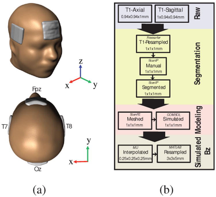
Model construction process used in the study. (a) Human head model, (b) Model construction flow diagram.

2) Phosphenes

Subjects were requested to report stimulation-related side effects while in the scanner. Phosphene perception was rated on a 1-10 scale, with 1 corresponding to ‘no detectable flashing’ and 10 corresponding to ‘white field’. Phosphene fields were recorded as either ‘peripheral’ or ‘central’. Subject perceptions of cutaneous stimulation were also recorded.

B. MR Imaging Procedures

All data were measured using a Philips 32-channel head coil in a 3 T MRI Philips Achieva scanner at the Advanced Magnetic Resonance Imaging and Spectroscopy Facility, UF McKnight Brain Institute. We gathered co-registered high resolution T₁ -weighted and diffusion weighted data on all subjects for computational model construction and comparison with MREIT results. MREIT acquisitions employed a Philips mffe protocol (Philips software version R3.2.1), modified to produce TTL-logic pulses after each MR excitation pulse, triggering a MR-safe battery-operated constant current source (DC-STIMULATOR MR, neuroConn, Ilmenau, Germany). Fig. 2(a) shows a schematic of the measurement setup. We verified that ‘no current’ (NC) measurements using the MREIT sequence did not affect processed signal phase [21]. In a separate experiment using agarose phantoms with known composition (Appendix), we verified that current-induced B_z maps were similar to model predictions.

Fig. 2.

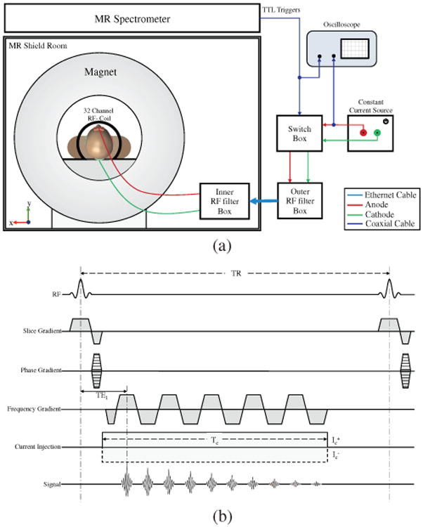
MRI setup and sequence used. (a) Experimental setup, (b) Multiecho fast field gradient echo (mffe) pulse sequence used in phantom and human volunteer experiments.

1) Structural Scans

After pilot scan acquisition, a 3D FLASH T₁ -weighted structural image was acquired with a 240 mm (FH) × 240 mm (AP) × 160 mm (RL) field-of-view (FOV) and 1 mm isotropic resolution, centered laterally on the mid-brain. Structural scans were processed using ScanIP (Synopsys, Exeter, UK) segmentation software to produce models with a uniform conductivity (σ = 1 S/m) and the same external shape as each subjects' head. Electrode locations and dimensions were also detected from T₁-weighted scans. The uniform model and electrodes were then meshed and exported to COMSOL (Burlington, MA). A forward problem was solved on this model using an input current density such that the total injected current at the anode was 1.5 mA. The cathode was set to ground potential. Current densities predicted within the model were sampled on a grid matched to the MREIT resolution and then converted to simulated B_z values using a FFT implementation of the Biot-Savart law [22]. Fig. 1(b) summarizes model construction steps.

2) tACS Magnetic Flux Density data collection (MREIT-CDI Scans)

Fig. 2(b) shows the Philips mffe sequence modified for MREIT-CDI. MREIT-CDI datasets were acquired in three 5 mm contiguous slices (NS = 3) with an in-plane FOV of 224 mm (RL) × 224 mm (AP) and a data matrix size 100 × 100 × 3 (resolution 2.24 × 2.24 × 5 mm³). MREIT-CDI slice positions were aligned to the T₁ -image volumes and chosen to encompass electrodes (Fig. 2(a)). MREIT-CDI scans were performed for each slice sequentially, and comprised 100 phase encode steps for each slice (PE = 100). For each PE step, ten echoes (NE = 10) were acquired during a current injection time (T_c) of 32 ms within a TR of 50 ms, then the current polarity was alternated during subsequent TR intervals. This sequence was repeated 12 times (NAV = 12) for each PE step. Therefore, the total acquisition time for each MREIT-CDI image was TR × 2 (polarity switching) × NAV × PE × NS = 6:00 minutes. The entire MREIT-CDI procedure was repeated, and the results averaged (a total acquisition time of 12 minutes) to achieve better signal-to-noise ratio (SNR) and to reduce standard deviations in current induced magnetic fields (B_z) [23]. An initial, no current (NC), MREIT scan was performed to verify system stability and produce baseline $T_2^{\ast }$ maps. Including averaging, NC scans required only 6 minutes since no polarity switching was used. The entire MREIT-CDI acquisition, comprising stimulation via both Fpz-Oz and T7-T8 electrode pairs and NC scans, lasted approximately 30 minutes. With polarity reversal every 50 ms, the MREIT-CDI protocol applied an alternating rectangular wave of 1.5-mA amplitude current and a full cycle length of 100 ms. Since the T_c was 32 ms in each 50 ms TR, the current injection duty cycle was approximately 64%. Fourier transformation of the current waveform showed maximum power at around 10 Hz (1/100 ms⁻¹).

3) Diffusion Weighted Imaging Scans and Tensor Reconstructions

Diffusion weighted MR (DWI) data was acquired using a HARDI (high angular resolution diffusion imaging) protocol, at b-values of 100 s/mm² (6 directions) and 1000 s/mm² (64 directions). Data were sampled at a 2 mm isotropic resolution, with a matrix size of 70 × 112 × 112. Two 6-direction DWI data sets were gathered with reversed phase encode directions to remove effects of background magnetic inhomogeneities. These two data sets were then combined using the FSL topup procedure [24]. While T₁ -weighted, MREIT and DWI data were all referred to the same reference scan, the S0 (no diffusion gradient, b = 0 s/mm²) DWI image registration was used to confirm alignment of T₁ -weighted and DTI data. Both the S0 and T₁-weighted images were then resampled to 100 × 100 × 44 matrix size to match MREIT-CDI resolution. Finally, DWI data were processed to tensors in FSL using the DTI-FIT command [25] to obtain six unique parameters describing each voxel as

$$\mathbf{D}=\left[\begin{array}{ccc}{D}_{xx}& D_{xy}& D_{xz}\\ D_{yx}& D_{yy}& D_{yz}\\ D_{zx}& D_{zy}& D_{zz}\end{array}\right]$$ (2)

where D_xy = D_yx, D_yz = D_zy, D_xz = D_zx.

C. Experimental Data Optimization and Processing

1) Phase Processing

MREIT: Positive and negative currents, denoted as $I_c^{+}$ and $I_c^{-}$, respectively, were applied to subjects in alternate TRs. The raw k-space data corresponding to each echo j, can be described by

$$S_j^{\pm }=\int \int {\rho }_j(x,y)e^{i{\delta }_j(x,y)}{e}^{\pm i\gamma {\widehat{B}}_z(x,y)T_{c,j}}{e}^{i2\pi (m\mathrm{\Delta }{k}_{x}x+n\mathrm{\Delta }{k}_{y}y)}dxdy$$ (3)

where ρ_j(x,y) is the MR signal at position x, y for the j^th echo, δ_j(x, y) represents a systematic background phase, γ is the gyromagnetic ratio of hydrogen, B̂_z(x,y) is the current induced magnetic flux density and T_c,j is the duration of the applied current at echo j. The complex-value image for each echo was obtained by discrete inverse Fourier transform of (3) to obtain complex images ${\rho }_j^{+}(x,y)$ and ${\rho }_j^{-}(x,y)$ where ${\rho }_j^{\pm }(x,y)$ corresponded to the images for application of positive or negative currents, respectively. Final magnetic flux density (B̂_z(x,y)) images were determined by complex division of images for positive and negative currents [9] as shown in (4) below.

$${\widehat{B}}_{z,j}(x,y)=\frac{1}{2\gamma T_{c,j}}arg\frac{{\rho }_j^{+}(x,y)}{{\rho }_j^{-}(x,y)}$$ (4)

2) B_z Optimization

Maps of $T_2^{\ast }$ distributions were generated for each slice using NC images. Optimal weighting factors (ω_j) for each echo [26] were then generated from these maps. The optimal B_z used for each montage was a weighted sum of the B̂_z,j for each echo as

$$B_z=\sum _{j=1}^{NE}{\omega }_j{\widehat{B}}_{z,j}.$$ (5)

As a final step, a ramp-preserving denoising preprocessing step [27] was applied to optimized data to improve overall SNR.

3) Phase and B_z Noise Floor Estimations

Underlying phase noise floor levels were computed using methods described in [23]. Experimental noise levels for each subject were computed inside manually selected white matter regions comprising at least 3000 voxels (Subject P1 3196 voxels, Subject P2 3456 voxels).

4) Projected Current Density Reconstruction

We adopted the method proposed by Park et al [28] to recover the current density from the z-component of the magnetic flux density (B_z). The recovered current density J^P from the measured B_z can be written as

$${\mathbf{J}}^P={\mathbf{J}}^0+\frac{1}{{\mu }_0}(\frac{\partial (B_z-B_z^0)}{\partial y},-\frac{\partial (B_z-B_z^0)}{\partial x},0)$$ (6)

where μ₀ = 4π × 10⁷ TmA⁻¹. Here, J⁰ is the current density developed in a homogeneous model of the imaged head, obtained by solving the Laplace equation subject to the same boundary conditions as in the experiment, and $B_z^0$ is the z-component of the magnetic flux density computed from the homogeneous model. The quality of conductivity tensor images recovered using DT-MREIT depends on how well the projected current J^P is recovered in the measured B_z data. To avoid propagation of noise from poor SNR regions (skull, and distortion near air-filled regions), we only reconstructed J^P distributions within a brain region of interest (ROI) free of distortion [29].

D. Anisotropic Conductivity Tensor Image Reconstruction

We determined the extra-cellular conductivity and diffusivity ratio map, denoted as η, using the reconstructed J^P and the water diffusion tensor maps. The position-dependent ratio η was determined by reconstructing J^P images from two linearly independent current injections, and solving the matrix system [17]

$$\left[\begin{array}{cc}{({\mathbf{D}}^{-1}{\mathbf{J}}^{P,1})}_y& -{({\mathbf{D}}^{-1}{\mathbf{J}}^{P,1})}_x\\ {({\mathbf{D}}^{-1}{\mathbf{J}}^{P,2})}_y& -{({\mathbf{D}}^{-1}{\mathbf{J}}^{P,2})}_x\end{array}\right]\left[\begin{array}{c}\frac{\partial ln\eta }{\partial x}\\ \frac{\partial ln\eta }{\partial y}\end{array}\right]\approx \left[\begin{array}{c}\frac{\partial {({\mathbf{D}}^{-1}{\mathbf{J}}^{P,1})}_x}{\partial y}-\frac{\partial {({\mathbf{D}}^{-1}{\mathbf{J}}^{P,1})}_y}{\partial x}\\ \frac{\partial {({\mathbf{D}}^{-1}{\mathbf{J}}^{P,2})}_x}{\partial y}-\frac{\partial {({\mathbf{D}}^{-1}{\mathbf{J}}^{P,2})}_y}{\partial x}\end{array}\right]$$ (7)

Although the scale factor ln η is formally recovered in (7) using D⁻¹, D is often ill-posed. Therefore, 0-th order Tikhonov regularization with an empirically determined regularization parameter of 0.01 was employed to suppress noise amplification. A detailed description of the image reconstruction procedure can be found in [17]. The anisotropic conductivity tensor distribution of the brain was obtained by multiplying the η value recovered for each voxel in the slice (i,j) by the diffusion tensor (equation (1)) to obtain

$$\begin{array}{c}{\mathbf{C}}_{i,j}={\eta }_{i,j}{\left[\begin{array}{ccc}{D}_{xx}& D_{xy}& D_{xz}\\ D_{yx}& D_{yy}& D_{yz}\\ D_{zx}& D_{zy}& D_{zz}\end{array}\right]}_{i,j}={\left[\begin{array}{ccc}{C}_{xx}& C_{xy}& C_{xz}\\ C_{yz}& C_{yy}& C_{yz}\\ C_{zx}& C_{zy}& C_{zz}\end{array}\right]}_{i,j}\end{array}$$ (8)

and C_xy = C_yx, C_yz = C_zy, C_xz = C_zx.

E. Quantitative Analysis

For quantitative analysis of reconstructed tissue conductivities, we assessed the conductivities of white matter (WM), gray matter (GM) and cerebrospinal fluid (CSF) in several 3 × 3 voxel ROIs. ROIs were identified by one author (MC) based on segmented T1 and DTI images, and results were analyzed by another (RJS). Differences between participant results were assessed quantitatively using t-tests (α < 0.05). Confirmations of ROI results were generated using independently segmented white matter, gray matter and CSF masks. For this bulk comparison, gray matter, white matter and CSF (P1 only) masks were segmented from T1-weighted data sets and co-registered with the central reconstructed conductivity slice for each participant. Conductivity eigenvalue images were multiplied by each mask, and modes of resulting datasets were computed. Modal values were chosen to avoid partial volume effects. ROI results were compared qualitatively with relevant literature values in the Discussion.

Data from two cylindrical phantoms of known conductivity composition were also collected and processed using the procedures detailed above, and used to confirm reconstruction accuracy and reproducibility. These data are presented in the Appendix.

III. Results

The T₁-weighted MR magnitude images were used to inform selection of white matter, gray matter and CSF ROIs. Fig. 3 shows T₁-weighted MR magnitude images, color-coded fractional anisotropy (FA) maps, MREIT magnitude images and segmented brain region masks for participants P1 and P2, respectively. The color-coded FA images illustrate directions of water diffusion within brain tissues, modulated by the degree of tissue anisotropy. Because WM is the most anisotropic tissue in the brain, it is highlighted in the images. Directions of principal eigenvectors in the diffusion map are indicated with a mix of colors signifying diffusion along the left-right (LR, red), posterior anterior (PA, green) or inferior-superior (IS, blue) axes. We also show (Fig. 3(c)) the 2.24 × 2.24 mm² resolution MREIT magnitude image that was co-registered to the 1 × 1 mm² T₁ -weighted images before construction of uniform conductivity computational models. Segmented brain masks used for J^P and η reconstructions are illustrated in Fig. 3(d)).

Fig. 3.

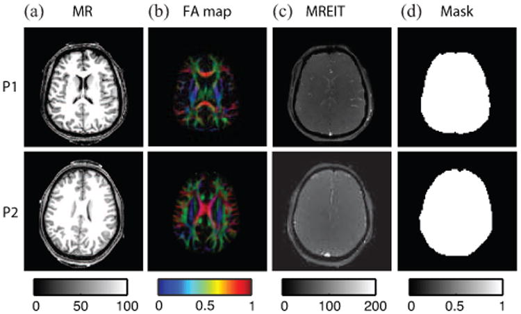
Image reference data for conductivity reconstruction process. (a) T₁ weighted MR image, (b) Color coded FA map, (c) MREIT magnitude image and (d) brain masks for P1 and P2.

The optimized magnetic flux density (B_z) images formed by 1.5 mA current injections used for reconstructing the anisotropic conductivity images are shown in Fig. 4(a) for each montage and subject. Baseline noise levels were of the order of 0.2 nA [21]. Corresponding projected current density (J^P) maps estimated from these B_z images using equation (6) are illustrated in Fig. 4(b). The η maps recovered by solution of (7) were reconstructed for both participants and are shown in Fig. 4(c). Note that reconstructed η maps depended upon both current density distributions and tissue types. High η values were found in CSF regions, as expected, and these regions are outlined in Fig. 4(c). Fig. 5 shows reconstructed MR magnitude, η and conductivity tensor images of two slices of each participant brain found using DT-MREIT methods.

Fig. 4.

Intermediate results of conductivity calculations. (a) Magnetic flux densities, (b) Computed Projected current densities and (c) calculated η distributions for participants (left) P1 and (right) P2. Boundaries of CSF regions detected in corresponding T1-weighted images are traced in red.

Fig. 5.

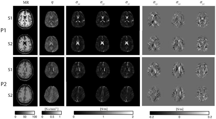
Magnitude, η and conductivity tensor images, shown by component, for participants (top) P1 and (bottom) P2.

Seven (P1) and six (P2) 3 × 3-voxel² (∼45 mm² area, 226 mm³ volume) ROIs were chosen in the conductivity tensor image of each participant. The three white matter ROIs were chosen such that principal fiber directions (as indicated by diffusion tensor images) were along the LR (x), PA (y) or IS (z) image directions for ROI 1, 2 and 3 respectively. Gray matter and CSF ROIs were chosen in locations with the largest uniform areas of each tissue type, although this was difficult for P2 in the case of CSF because the slice chosen contained only small contiguous volumes of CSF. Therefore, only one CSF ROI was located for P2. ROI locations (numbered 1-3 in white matter, 4 and 5 in gray matter, 6 or 7 in CSF), are shown for each participant in Fig. 6(a). Average values of diagonal components (C_xx, C_yy and C_zz) of reconstructed anisotropic conductivity tensors in each ROI are plotted, with 95% confidence intervals, in Fig. 6(b). In Fig. 6(b), diagonal tensor components for participants P1 and P2 are represented by circles (○) and squares (□), respectively. Average eigenvalues over each ROI are shown with 95% confidence intervals (CI) in Fig. 6(c).

Fig. 6.

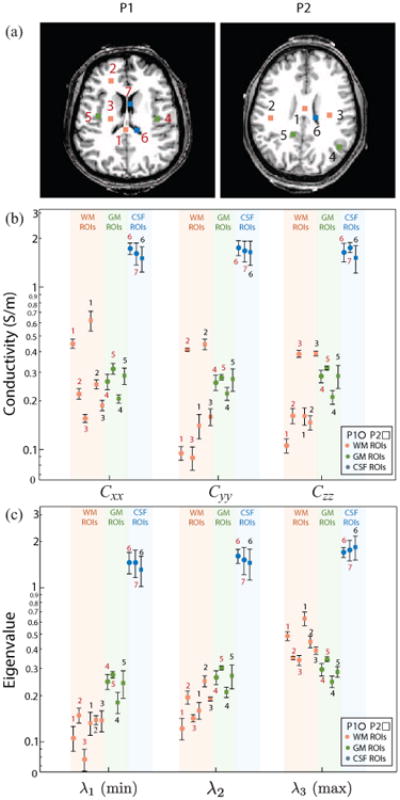
ROI locations, diagonal reconstructed conductivity tensor components and eigenvalues of conductivity tensors for each participant. (a) ROI locations 1-3 (WM), 4-5 (GM) and 6-7 (CSF) for P1 (red) and P2 (black), (b) Diagonal conductivity tensor entries for each subject in each ROI, with 95% confidence intervals. P1 ROIs are indicated with red numbers and ○ symbols, P2 ROIs are indicated with black numbers and □ symbols. WM ROIs were chosen such that principal eigenvectors were in LR, PA and SI directions respectively, (c) Conductivity tensor eigenvalues, with 95% confidence intervals. Here λ₃ is the principal (maximum) eigenvalue for each ROI and participant.

For P1 and P2, we found average principal WM eigenvalues (λ₃) of 0.391 S/m ([0.361, 0.421] 95% CI) and 0.489 S/m ([0.441, 0.538]) respectively. The average ratio between λ₃ and pooled λ₁ or λ₂ values was 3.397 ([2.985, 3.810]) for P1, and 3.179 ([2.832, 3.525]) for P2. Mean transverse eigenvalues (λ₁, λ₂) were 0.132 S/m ([0.120, 0.144]) for P1 and 0.168 S/m ([0.155, 0.181]) for P2.

Gray matter ROIs were approximately isotropic (FA≤ 0.2) and we found averaged pooled eigenvalues were around 0.287 S/m ([0.275, 0.300]) for P1 and 0.238 S/m ([0.222, 0.255]) for P2.

In CSF ROIs, average fractional anisotropy values of around 0.105 were found in P1, and 0.187 was found in P2. No significant differences in CSF diagonal tensor elements or eigenvalues were found between the three CSF ROIs considered. Average eigenvalues for CSF ROIs were 1.583 S/m ([1.482, 1.684]) and 1.532 S/m ([1.328, 1.737]) for P1 and P2 respectively.

Results showing modal conductivity eigenvalues in bulk gray matter, white matter and CSF (P1) are summarized in Table I. Modal eigenvalues were similar to ROI values, confirming that our chosen ROIs were representative of data overall. We therefore continued analyses using ROI data.

Table I.

Modal conductivity eigenvalues (S/m) in white matter, gray matter and CSF masks (P1 only) in central reconstructed DT-MREIT images. Numbers of voxels in each mask are also noted.

Participant	WM			GM			CSF
	λ1	λ2	λ3	λ1	λ2	λ3	λ1	λ2	λ3
P1	0.13	0.19	0.32	0.28	0.31	0.28	1.59	1.69	1.54
# voxels		821			149			44
P2	0.15	0.26	0.34	0.28	0.34	0.37	-	-	-
# voxels		1085			95			-

A. Differences Between Participant Conductivity Values

Results found in the white matter, gray matter and CSF ROIs of the two participants were similar overall. CSF values in ROIs were not significantly different (α=0.6139). Averaged gray matter conductivity values were significantly higher in P1, but average, transverse and longitudinal white matter conductivities were significantly higher in P2.

B. Subject Phosphene Perceptions

Both subjects reported phosphene occurrence in peripheral fields for both montages. The Fpz-Oz montage was perceived to produce more intense phosphenes than T7-T8. Subject P1 reported an intensity of 3.5 out of 10 for the T7-T8 montage and 4 for Fpz-Oz. Subject P2 perceived intensities of 4 and 7 for the T7-T8 and Fpz-Oz montages respectively. Phosphene locations reported by Subject P2 during Fpz-Oz stimulation were described as being above the eyes and near the Fpz location. Both subjects reported cutaneous perceptions as slight tingling sensations centered on electrode locations.

IV. Discussion

The images presented here represent the first in vivo conductivity images of the human brain, reconstructed using DT-MREIT techniques. The measurements recovered here provide conductivity values applicable to signals at brain activity frequencies. These measurements therefore have relevance to construction of accurate forward models for source imaging. They may also be of use in detection of pathology (for example, cancerous tissues show typically higher conductivities [30]). In the following sections we compare the values measured here with those reported in other contexts and studies. A summary of this survey is presented in Table II below. In Table II, tissue conductivities cited were measured in vivo, at body temperature and at 10 Hz unless otherwise specified. In the case of both [8] and [11], results from two subjects were reported, and values for each subject are reported for each tissue type. Measurements of longitudinal (l), transverse (t) and average (av.) white matter conductivities were included where possible. Average tissue conductivity values quoted in Table II for this study and [11] were found by computing mean eigenvalues over all ROIs. ‘Average’ white matter conductivities in Table II for other studies are values reported without reference to measurement geometry at low frequencies, or reported at high frequencies [8] where tissue is effectively isotropic.

Table II.

Comparison of conductivities (S/m) measured using MREIT at 10 Hz to related literature values.

Tissue	hoc op.	[31]	[32]–[34]a	[8]b	[11]c	[35]d
CSF	1.583, 1.532	1.55e	-	1.56, 1.27	1.3, 1.3	1.79
GM	0.287, 0.239	0.23f	0.03	0.69, 0.67	0.36, 0.34	-
WM (l)	0.391, 0.490	0.47g	-	-	0.88, 0.56	-
(t)	0.132, 0.168	0.08g	-	-	0.46, 0.26	-
(av)	0.218, 0.275	0.10h, 0.13f	0.03	0.46, 0.38	0.60, 0.36	-

^aBovine samples

^bHuman, 298 MHz, 2 subjects

^cCanine, ∼5 Hz, 2 subjects

^dHuman samples

^eHuman sample, 1 kHz, 25°C [36]

^fRabbit samples, 1 kHz [38]

^gCat (spinal cord), 5-10 Hz [39]

^hRabbit, 1 kHz [40]

A. Comparison to specific conductivity measurements

Many values in the literature are from direct 2- or 4-terminal impedance measurements on excised tissues or fluids, or anesthetized animals. Tissue conductivity values most often used in computational models or cited in the literature are typically drawn from Geddes and Baker [31] or Gabriel et al. [32]–[34]. CSF conductivity values are frequently sourced from Baumann et al. [35].

Values found in the literature survey of Geddes and Baker [31] were remarkably consistent with those found here overall. However, none of the measurements cited in [31] matched the conditions of this study exactly. The study of Radvan-Ziemnowicz [36] was performed at 24.5 °C. Conductivities of body tissues typically increase at around 2%/ °C [37], therefore while the values found in this work correspond well, it would be expected that conductivity of CSF samples at human body temperature would have been approximately 2 S/m. The gray matter conductivity cited in [38] was obtained immediately post mortem (within one hour) in rabbit tissue at a frequency of 1 kHz. Use of a higher frequency may have resulted in a slightly higher conductivity reading, and while the study reported no evidence of conductivity change in the first hour post mortem, values typically increase as tissue undergoes initial postmortem changes. The most comparable study cited in [31] came from Ranck and BeMent [39], where conductivity measurements were performed on anesthetized cats that had undergone laminectomy. While spinal cord tissue was sampled, frequencies of 5-10 Hz were employed, and results were qualitatively similar to those found here. Average or effective isotropic white matter conductivities were reported in both [38] and [40], for rabbit tissue at 1 kHz. In the case of [40] recordings were made in vivo. Both measurements were lower than found here.

Comparison with Gabriel et al. [32]–[34] was only possible for two tissues, white and gray matter. The original measurements reported in [32]–[34] at 10 Hz were from bovine tissue samples, and showed a much lower gray matter or effective isotropic white matter conductivity than found here. We note that the conductivity values we found were closer to those shown overlaid in the figures of [32]–[34] (not directly cited), at higher frequencies (>10 kHz), that were found in their literature searches.

In Baumann et al. [35], CSF conductivity values were recorded in seven previously stored samples of CSF, warmed to an approximate body temperature of 37 °C, at a range of frequencies between 10 Hz and 10 kHz. At 10 Hz and 37 °C, CSF conductivity was measured to be 1.789 ± 0.018 S/m (x̄±sd). This was higher than conductivities recorded in CSF ROIs in this study. This may be related to the choice of ROI in this work (and the possible influence of partial volumes of other tissues), the effect of storage on samples in [35], and possibly the source of samples in [35] (neurosurgical patients).

B. Comparison to EPT results

It is also possible to qualitatively compare conductivity values found here with those found in another study [8] performed using EPT at 7T, which corresponds to a measurement frequency of about 298 MHz. Since EPT cannot assess anisotropy information, we compare the values in [8] with averaged white matter conductivities found in this study. Complex tissue conductivities increase as a function of frequency [34], [37], so we would expect EPT-derived conductivities to be higher than those found at 10 Hz. The lower white matter conductivity values of around 0.25 S/m found in this study are therefore consistent with values of around 0.4 S/m measured at 298 MHz. Similarly, the gray matter conductivity values of around 0.26 S/m found here are compatible with the values of around 0.68 S/m found using EPT. Since CSF is principally an electrolytic fluid and demonstrates a typically flat conductivity profile [31], [35], a direct comparison can be made with [8]. Again, the conductivities of approximately 1.5 S/m found were consistent with values found in [8].

C. Comparison to other DT-MREIT results

The closest possible match to the experimental conditions of the present study is the study of Jeong et al. [11]. Their study was performed on two canine subjects, with an MREIT sequence TR of 200 ms, corresponding to a stimulation frequency of approximately 5 Hz. They obtained broadly similar results to ours, but CSF conductivities were lower. Both gray and white matter conductivities were higher overall in their study. It is not clear if this was the result of interspecies difference or choice of ROI locations.

D. Differences Between Participants

Results from ROI calculations showed that CSF values were not significantly different for P1 and P2 samples. However, gray matter conductivities were significantly higher in P1, and white matter conductivities were overall higher for P2. Because of the limited sampling, both in brain coverage and in number of ROIs considered, it was not possible to determine if differences between tissues were characteristic of the brain slice or structures sampled in each participant, or of true differences between participants. Further analysis of conductivities over entire brains, with a larger number of participants, will enable a more comprehensive assessment of variability in tissue conductivities.

E. Phosphene Perceptions

Transcutaneous stimulation at frequencies up to 80 kHz has been reported to induce phosphenes [41], with a minimum threshold of perception at around 10 Hz [42], [43]. Because stimulation was applied here at 10 Hz, it is therefore not surprising that subjects perceived phosphenes. Some level of phosphene perception or cutaneous tingling sensations at electrode locations have been commonly reported in tES recipients, and are not considered to be a safety issue [44]. While phosphenes in tDCS may be avoided by slowly ramping current intensity [45], this strategy was not possible in our experiment. The higher phosphene perception ratings for the Fpz-Oz montage may have been because the stimulating electrodes were closest to the retina and occipital lobe respectively [46], [47].

F. Improved in vivo MREIT techniques

In this study we presented conductivity reconstructions of two 5 mm-thick slices of each participant's brain. It would be an advantage to measure the brain conductivity more completely by sampling the brain more completely and with a higher resolution. Because the sequences used here involved MREIT acquisitions of approximately 18 minutes each, faster sequences must be used to avoid fatiguing subjects. We have now developed echo planar imaging (EPI) MR methods that can be used to sample brain information more rapidly [48], and introduced new undersampling techniques [49]. In addition, new fast multi-band SENSE imaging techniques [50] should allow more rapid sampling of the brain. We intend to explore these methods further in subsequent studies.

V. Conclusion

DT-MREIT measurements of in vivo conductivity distributions within the brains of two human subjects were recovered. Results were consistent with those found in relevant literature. Future studies involving more brain coverage will enable a more detailed assessment of tissue conductivities by type and structure. These measurements will potentially be of great use in assessment of brain pathology, and in inverse EEG modeling.

Appendix.

Two confirmatory experiments were performed using agar-based phantoms to determine the reproducibility and accuracy of reconstructed DT-MREIT conductivities. A two-part cylindrical phantom (Phantom A), and a one-part cylindrical phantom (Phantom B) were constructed and imaged using the same protocol as used in the experiments of the main paper. Both phantoms were the same size and shape. Phantom A consisted of a background material of approximately 0.5 S/m conductivity and a central inclusion with ∼1.6 S/m conductivity. Phantom B consisted only of background material. Multiple imaging runs were performed on each phantom to investigate reproducibility. Reconstructed conductivities were compared with four-terminal conductivity measurements performed on separate bulk samples of each phantom material.

A. Phantom Description

Both phantoms were approximately 100 mm in diameter and 120 mm high. The size and shape of Phantom A is illustrated in schematic form in Fig. A.1 below, showing the approximately 40 mm-diameter cylindrical inclusion. Compositions and approximate conductivities of the two materials used in Phantoms A and B are shown in Table A.1.

B. Phantom Imaging Procedures

Imaging of both phantoms was performed using methods identical to those described in the main text. That is, we first performed structural T1-weighted FLASH imaging of the phantom followed by DTI imaging. We then used the mffe sequence to measure phase for each diametric pair of electrodes. In the in vivo work described in the main text, data were averaged over two runs for each electrode pair for each subject. However, in phantom experiments, 10 MREIT runs for each electrode pair were collected, covering a period of approximately 200 min after phantom construction. Data from neighboring pairs of runs were averaged into five sets of data for each electrode pair. This procedure was performed to investigate stability of reconstructed conductivity values. The imaging parameters and fields of view used for phantoms were identical to those used in human studies.

Fig. A.1.

Oblique and Cross-sectional views of phantom. (left) Oblique, showing surface electrode placement. Phantom height was 120 mm. (right) Top view of phantom. Overall diameter was 100 mm, inclusion diameter was 40 mm.

C. Phantom Image Reconstruction

The T1-weighted structural images were segmented and current densities in a uniform object with the same external shape as the phantom were simulated using COMSOL. Conductivity reconstructions were performed with optimized, weighted MREIT data, using identical methods and the same reconstruction parameters as for in vivo images. Reconstruction accuracy was assessed by comparing reconstructed values for the background and inclusion of Phantom A, and the background material of Phantom B, with those found using four terminal impedance measurement.

Reconstructed mean conductivities (MC) in each image were computed via

$$MC=\frac{{\lambda }_1+{\lambda }_2+{\lambda }_3}{3}$$ (9)

where λ₁, λ₂ and λ₃ were principal conductivity eigenvalues.

ROIs inside the inclusion and background respectively were identified from MREIT magnitude images. MC values within these ROIs were compared with four-terminal conductivity measurements performed on separate samples of inclusion and background materials. We performed t-tests to determine if differences between independently measured conductivities and reconstructed conductivities were significant, with significance set at α <0.05.

D. Independent Conductivity Determination

Four-terminal conductivity measurements were performed on five individually mixed hexahedral-shaped samples of inclusion and background material. A low-frequency impedance analyzer (HP 4192A, Hewlett Packard, Palo Alto, CA) was used to measure resistances. The mean conductivity of inclusion material was 1.6 S/m and for the background material the mean was 0.5 S/m. These values are shown in Table A. 1 with 95% confidence intervals.

Fig. A.2.

MREIT Magnitude, phase images and corresponding reconstructed conductivity parameters for each data set for Phantom A. (a) MREIT magnitude images and phase images for left-right (LR) and top-bottom (TB) current flow, (b) reconstructed η values and (c) reconstructed conductivity eigenvectors and MC.

E. Conductivity Reconstructions

Phase and reconstructed conductivity parameters for Phantom A are summarized in Fig. A. 2 below. Both phantoms were identified as isotropic, since fractional anisotropy values throughout phantoms were < 0.05. Measurements of Phantom A conductivities were affected by osmotic diffusion between the two materials [51].

Conductivity of the inclusion decreased from around 1.6 S/m to 1.4 S/m over the course of the experiment and background material ROI increased from 0.6 S/m to 0.64 S/m. Phantom A background material conductivities were consistently higher than found in independent conductivity measurements, most likely because of osmotic diffusion of salt from the high-conductivity inclusion to the background material.

Phantom B reconstructions were stable over multiple runs, with an average reconstructed conductivities in a central ROI averaging 0.501 S/m.

Fig. A.3.

Plot of independently determined mean conductivities and 95% confidence intervals for background (green shading) and inclusion (red shading) materials, compared with MC value confidence intervals in reconstructed ROIs of Phantoms A and B. Insets show locations of inclusion (green) and background (red) ROIs in Phantom A (left) and background material ROI in Phantom B (right).

F. Conductivity Reproducibility

Independent conductivity measurements and reconstructed conductivities are compared in Fig. A. 3. We saw that mean and 95% confidence intervals in reconstructed conductivities of Phantom B were similar for all 5 sets of data, neglecting effects caused by diffusion. Correlation coefficients were calculated between all pairs of Phantom B ROI data sets using the MATLAB command corrcoeff. All sets of Phantom B ROI data were found to be not significantly different, except for comparison of Sets 3 and 5.

G. Conductivity Accuracy

Two-sample t-tests comparing MC ROI data within the inclusion of Phantom A with independently measured inclusion conductivities showed reconstructed conductivities were not significantly different from the independent four-terminal conductivity measurements for all cases except Set 5. There were significant differences between conductivities in all reconstructed sets and independent measurements for the background material in Phantom A, but we believe this was due to significant mixing of inclusion and background materials.

Conductivity accuracy analyses must take into account the possibility that in-magnet and laboratory data were collected with samples at different temperatures, since electrolyte solution conductivity increases by approximately 2 %/°C [37]. The best comparison of reconstructed and independently measured conductivity is provided by Phantom B data. Background MC values in Phantom B were lower than those measured in Phantom A, averaging 0.487 S/m over all five runs, and had smaller confidence intervals due to the lack of osmotic diffusion processes. The temperature measured in the magnet bore during Phantom B imaging was 21.0 ± 0.3 °C. The average conductivity of background materials, measured at a laboratory temperature of 24 °C, was 0.501 S/m. The predicted Phantom B reconstructed conductivity at 24 °C is 0.507 S/m, only 1 % greater than those measured in the laboratory, thus confirming reconstruction accuracy.

Table A.1.

Composition of background and inclusion materials. Confidence intervals of measured phantom material conductivities are shown next to mean values.

Quantity	Background	Inclusion
Water (ml)	1000	1000
Agar (g)	25	25
NaCl (g)	1	6
CuSO4 (g)	0.25	0.25
Measured Conductivity (S/m)	0.50 [0.46, 0.54]	1.59 [1.56, 1.62]

References

- 1.Hallez H, Vanrumste B, Grech R, Muscat J, De Clercq W, Vergult A, D'Asseler Y, Camilleri KP, Fabri S, Van Huffel S, Lemahieu I. Review on solving the forward problem in EEG source analysis. Journal of NeuroEngineering and Rehabilitation. 2007;4:46. doi: 10.1186/1743-0003-4-46. [DOI] [PMC free article] [PubMed] [Google Scholar]
- 2.Sadleir RJ, Vannorsdall TD, Schretlen DJ, Gordon B. Target optimization in transcranial direct current stimulation. Frontiers in Psychiatry. 2012;3:90. doi: 10.3389/fpsyt.2012.00090. [DOI] [PMC free article] [PubMed] [Google Scholar]
- 3.Holder D. Electrical Impedance Tomography Methods, history and applications. 1st. Bristol and Philadelphia: Institute of Physics Publishing; 2005. ser. Series in Medical Physics and Biomedical Engineering. [Google Scholar]
- 4.Sylvester J, Uhlmann G. A global uniqueness theorem for an inverse boundary value problem. Annals of Mathematics. 1987;125:153–169. [Google Scholar]
- 5.Sadleir RJ, Tang T. Electrode configurations for detection of intraventricular haemorrhage in the premature neonate. Physiological Measurement. 2009;30(1):63–79. doi: 10.1088/0967-3334/30/1/005. [DOI] [PMC free article] [PubMed] [Google Scholar]
- 6.Aristovich KY, Packham BC, Koo H, Dos Santos GS, Mc Evoy A, Holder D. Imaging fast elecrical activity in the brain with electrical impedance tomography. NeuroImage. 2016;124:204–213. doi: 10.1016/j.neuroimage.2015.08.071. [DOI] [PMC free article] [PubMed] [Google Scholar]
- 7.Voigt T, Katscher U, Doessel O. Quantitative conductivity and permittivity imaging of the human brain using electric properties tomography. Magnetic Resonance in Medicine. 2011;66:456–466. doi: 10.1002/mrm.22832. [DOI] [PubMed] [Google Scholar]
- 8.Liu J, Zhang X, Schmitter S, Van de Moortele PF, He B. Gradient-based electrical properties tomography gEPT): a robust method for mapping electrical properties of biological tissues in vivo using magnetic resonance imaging. Magnetic Resonance in Medicine. 2015;74:634–646. doi: 10.1002/mrm.25434. [DOI] [PMC free article] [PubMed] [Google Scholar]
- 9.Seo JK, Woo EJ. Electrical tissue property imaging at low frequency using MREIT. IEEE Transactions on Biomedical Engineering. 2014;61(5):1390–1399. doi: 10.1109/TBME.2014.2298859. [DOI] [PubMed] [Google Scholar]
- 10.Kwon O, Sajib SZK, Sersa I, Oh TI, Jeong WC, Kim HJ, Woo EJ. Current density imaging during transcranial direct current stimulation (tDCS) using DT-MRI and MREIT: Algorithm develoment and numerical simulations. IEEE Transactions on Biomedical Engineering. 2015 doi: 10.1109/TBME.2015.2448555. [DOI] [PubMed] [Google Scholar]
- 11.Jeong WC, Sajib SZK, Katoch N, Kim HJ, Kwon O, Woo EJ. Anisotropic conductivity tensor imaging of canine brain using DT-MREIT. IEEE Transactions on Medical Imaging, pp. 2016:1–8. doi: 10.1109/TMI.2016.2598546. [DOI] [PubMed] [Google Scholar]
- 12.Joy M, Scott G, Henkelman M. In vivo detection of applied electric currents by magnetic resonance imaging. Magnetic Resonance Imaging. 1989;7(1):89–94. doi: 10.1016/0730-725x(89)90328-7. [Online] Available: http://www.sciencedirect.com/science/article/pii/0730725X89903287. [DOI] [PubMed] [Google Scholar]
- 13.Scott GC, Joy MLG, Armstrong RL, Henkelman RM. Measurement of nonuniform current density by magnetic resonance. IEEE Transactions on Medical Imaging. 1991;10:362–374. doi: 10.1109/42.97586. [DOI] [PubMed] [Google Scholar]
- 14.Scott GC, Joy MLG, Armstrong RL, Henkelman RM. Sensitivity of magnetic-resonance current-density imaging. Journal of Magnetic Resonance. 1992;97:235–254. [Google Scholar]
- 15.Tuch DS, Weeden VJ, Dale AM, George JS, Belliveau JW. Conductivity mapping of biological tissue using diffusion MRI. Annals of the New York Academy of Sciences. 1999;888(1):314–316. doi: 10.1111/j.1749-6632.1999.tb07965.x. [Online] Available: http://dx.doi.org/10.1111/j.1749-6632.1999.tb07965.x. [DOI] [PubMed] [Google Scholar]
- 16.Tuch DS, Wedeen VJ, Dale AM, George JS, Belliveau JW. Conductivity tensor mapping of the human brain using diffusion tensor MRI. Proceedings of the National Academy of Science USA. 2001;98:11 697–11 701. doi: 10.1073/pnas.171473898. [DOI] [PMC free article] [PubMed] [Google Scholar]
- 17.Kwon OI, Jeong WC, Sajib SZK, Kim HJ, Woo EJ. Anisotropic conductivity tensor imaging in MREIT using directional diffusion rate of water molecules. Physics in Medicine and Biology. 2014;59(12):2955. doi: 10.1088/0031-9155/59/12/2955. [Online] Available: http://stacks.iop.org/0031-9155/59/i=12/a=2955. [DOI] [PubMed] [Google Scholar]
- 18.Ma W, DeMonte TP, Nachman AI, Elsaid NMH, Joy MLG. Experimental implementation of a new method of imaging anisotropic electric conductivities; 2013 35th Annual International Conference of the IEEE Engineering in Medicine and Biology Society (EMBC); Jul, 2013. pp. 6437–6440. [DOI] [PubMed] [Google Scholar]
- 19.Folstein MF, Folstein SE, McHugh PR. “Mini-mental state” A practical method for grading the cognitive state of patients for the clinician. Journal of Psychiatric Research. 1975;12(3):189–198. doi: 10.1016/0022-3956(75)90026-6. [Online] Available: http://dx.doi.org/10.1016/0022-3956(75)90026-6. [DOI] [PubMed] [Google Scholar]
- 20.Oldfield RC. The assessment and analysis of handedness: the Edinburgh inventory. Neuropsychologia. 1971;9:97–113. doi: 10.1016/0028-3932(71)90067-4. [DOI] [PubMed] [Google Scholar]
- 21.Kasinadhuni AK, Indahlastari A, Chauhan M, SchŁr M, Mareci TH, Sadleir RJ. Imaging of current flow in the human head during transcranial electrical therapy. Brain Stimulation. 2017;10:764–772. doi: 10.1016/j.brs.2017.04.125. [DOI] [PMC free article] [PubMed] [Google Scholar]
- 22.Minhas A, Kim HH, Meng ZJ, Kim YT, Kim HJ, Woo EJ. Three-dimensional MREIT simulator of static bioelectromagnetism and MRI. Biomedical Engineering Letters. 2011;1:129–136. [Google Scholar]
- 23.Sadleir RJ, Grant S, Zhang SU, Lee BI, Pyo HC, Oh SH, Park C, Woo EJ, Lee SY, Kwon O, Seo JK. Noise analysis in magnetic resonance electrical impedance tomography at 3 and 11 T field strengths. Physiological Measurement. 2005;26:875–884. doi: 10.1088/0967-3334/26/5/023. [DOI] [PubMed] [Google Scholar]
- 24.Andersson JL, Skare S, Ashburner J. How to correct susceptibility distortions in spin-echo echo-planar images: application to diffusion tensor imaging. Neuroimage. 2003;20:870–88. doi: 10.1016/S1053-8119(03)00336-7. [DOI] [PubMed] [Google Scholar]
- 25.Jenkinson M, Beckmann CF, Behrens TE, Woolrich MW, Smith SM. FSL. NeuroImage. 2012;62:782–790. doi: 10.1016/j.neuroimage.2011.09.015. [DOI] [PubMed] [Google Scholar]
- 26.Oh TI, Jeong WC, Kim JE, Sajib SZ, Kim HJ, Kwon OI, Woo EJ. Noise analysis in fast magnetic resonance electrical impedance tomography (MREIT) based on spoiled multi gradient echo (SPMGE) pulse sequence. Phys Med Biol. 2014;59:4723–38. doi: 10.1088/0031-9155/59/16/4723. [DOI] [PubMed] [Google Scholar]
- 27.Lee CO, Jeon KAS, Ahn S, Kim HJ, Woo EJ. Ramp-preserving denoising for conductivity image reconstruction in magnetic resonance electrical impedance tomography (MREIT) IEEE Transactions on Biomedical Engineering. 2011;58(7):2038–2050. doi: 10.1109/TBME.2011.2136434. [DOI] [PubMed] [Google Scholar]
- 28.Park C, Lee BI, Kwon O. Analysis of recoverable current from one component of magnetic flux density in MREIT and MRCDI. Physics in Medicine and Biology. 2007;52:3001–3013. doi: 10.1088/0031-9155/52/11/005. [DOI] [PubMed] [Google Scholar]
- 29.Sajib SZK, Kim HJ, Kwon O, Woo EJ. Regional absolute conductivity reconstruction using projected current density in MREIT. Physics in Medicine and Biology. 2012;57:5841–5859. doi: 10.1088/0031-9155/57/18/5841. [DOI] [PubMed] [Google Scholar]
- 30.Surowiec AJ, Stuchly SS, Barr JR, Swarup A. Dielectric properties of breast carcinoma and the surrounding tissues. IEEE Transactions on Biomedical Engineering. 1988;35:257–263. doi: 10.1109/10.1374. [DOI] [PubMed] [Google Scholar]
- 31.Geddes L, Baker LE. The specific resistance of biological materials: a compendium of data for the biomedical engineer and physiologist. Medical & Biological Engineering and Computing. 1967;5:271–293. doi: 10.1007/BF02474537. [DOI] [PubMed] [Google Scholar]
- 32.Gabriel C, Gabriel S, Corthout E. The dielectric properties of biological tissues: I. Literature survey. Physics in Medicine and Biology. 1996;41:2231–2249. doi: 10.1088/0031-9155/41/11/001. [DOI] [PubMed] [Google Scholar]
- 33.Gabriel S, Lau RW, Gabriel C. The dielectric properties of biological tissues: II. Measurements in the frequency range 10 Hz to 20 GHz. Physics in Medicine and Biology. 1996;41:2251–2269. doi: 10.1088/0031-9155/41/11/002. [DOI] [PubMed] [Google Scholar]
- 34.Gabriel S, Lau RW, Gabriel C. The dielectric properties of biological tissues: III. Parametric models for the dielectric spectrum of tissues. Physics in Medicine and Biology. 1996;41:2271–2293. doi: 10.1088/0031-9155/41/11/003. [DOI] [PubMed] [Google Scholar]
- 35.Baumann SB, Wozny DR, Kelly SK, Meno FM. The electrical conductivity of human cerebrospinal fluid at body temperature. IEEE Transactions on Biomedical Engineering. 1997;44:220–223. doi: 10.1109/10.554770. [DOI] [PubMed] [Google Scholar]
- 36.Radvan-Ziemnowicz SA, McWilliams JC, Kucharski WE. Conductivity versus frequency in human and feline cerebrospinal fluid. In: Werner, editor. Proc 17th Ann Conf Eng Med Biol. Vol. 6. 1964. p. 108. Conference Proceedings. [Google Scholar]
- 37.Grimnes S, Martinsen OG. Bioimpedance & Bioelectricity Basics. 1st. London, San Diego: Academic Press; 2000. [Google Scholar]
- 38.Crile GW, Hosmer HR, Rowland AF. The electrical conductivity of animal tissues under normal and pathological conditions. American Journal of Physiology. 1922;60:59–106. [Google Scholar]
- 39.Ranck JB, BeMent SL. The specific impedance of the dorsal columns of cat: an anisotropic medium. Experimental Neurology. 1965;11:451–463. doi: 10.1016/0014-4886(65)90059-2. [DOI] [PubMed] [Google Scholar]
- 40.van Harreveld A, Murphy T, Nobel KW. Specific impedance of rabbit's cortical tissue. American Journal of Physiology. 1963;205:203–207. doi: 10.1152/ajplegacy.1963.205.1.203. [DOI] [PubMed] [Google Scholar]
- 41.Antal A, Paulus W. Transcranial alternating current stimulation (tACS) Frontiers in Human Neuro-science. 2013;7(317) doi: 10.3389/fnhum.2013.00317. [Online] Available: http://journal.frontiersin.org/article/10.3389/fnhum.2013.00317. [DOI] [PMC free article] [PubMed] [Google Scholar]
- 42.Lövsund P, Öburg PÅ, Nilsson S. Magneto- and electrophosphenes: a comparative study. Medical & Biological Engineering and Computing. 1980;18(6):758–764. doi: 10.1007/BF02441902. [DOI] [PubMed] [Google Scholar]
- 43.Kanai H, Chaieb L, Antal A, Walsh V, Paulus W. Frequency-dependent electrical stimulation of the visual cortex. Current Biology. 2008;18:1839–1843. doi: 10.1016/j.cub.2008.10.027. [DOI] [PubMed] [Google Scholar]
- 44.Bikson M, Grossman P, Thomas C, Zannou AL, Jiang J, Adnan T, Mourdoukoutas AP, Kronberg G, Truong D, Boggio P, Brunoni AR, Charvet L, Fregni F, Fritsch B, Gillick B, Hamilton RH, Hampstead BM, Jankord R, Kirton A, Knotkova H, Liebetanz D, Liu A, Loo C, Nitsche MA, Reis J, Richardson JD, Rotenberg A, Turkeltaub PE, Woods AJ. Safety of transcranial direct current stimulation: Evidence based update 2016. Brain Stimulation: Basic, Translational, and Clinical Research in Neuromodulation. 2016;9(5):641–661. doi: 10.1016/j.brs.2016.06.004. [Online] Available: http://dx.doi.org/10.1016/j.brs.2016.06.004. [DOI] [PMC free article] [PubMed] [Google Scholar]
- 45.Woods A, Antal A, Bikson M, Boggio PS, Brunoni AR, Celnik P, Cohen L, Fregni F, Herrmann CS, Kappenman ES, Knotkova H, Liebetanz D, Miniussi C, Miranda PC, Paulus W, Priori A, Reato D, Stagg C, Wenderoth N, Nitsche M. A technical guide to tDCS, and related non-invasive brain stimulation tools. Clinical Neurophysiology. 2016;127:10311048. doi: 10.1016/j.clinph.2015.11.012. [DOI] [PMC free article] [PubMed] [Google Scholar]
- 46.Paulus W. On the difficulties of separating retinal from cortical origins of phosphenes when using transcranial alternating current stimulation (tACS) Clinical Neurophysiology. 2010;121:987–991. doi: 10.1016/j.clinph.2010.01.029. [DOI] [PubMed] [Google Scholar]
- 47.Laakso I, Hirata A. Computational analysis shows why transcranial alternating current stimulation induces retinal phosphenes. Journal of Neural Engineering. 2013;10(4):046009. doi: 10.1088/1741-2560/10/4/046009. [DOI] [PubMed] [Google Scholar]
- 48.Chauhan M, Vidya Shankar R, Ashok Kumar N, Kodibagkar V, Sadleir RJ. Multi-shot echo-planar MREIT for fast imaging of conductivity, current density and electric field distributions. Magnetic Resonance in Medicine. 2018;79:71–82. doi: 10.1002/mrm.26638. [DOI] [PMC free article] [PubMed] [Google Scholar]
- 49.Song Y, Seo JK, Chauhan M, Ashok Kumar N, Sadleir RJ. Fast, adaptive acquisition strategies for low-frequency conductivity imaging using MREIT. Physics in medicine and biology. 2018;63:045011. doi: 10.1088/1361-6560/aaa8d2. [DOI] [PMC free article] [PubMed] [Google Scholar]
- 50.Moeller S, Yacoub E, Olman CA, Auerbach E, Strupp J, Harel N, Ugurbil K. Multiband multislice GE-EPI at 7 Tesla, with 16-fold acceleration using partial parallel imaging with application to high spatial and temporal whole-brain fMRI. Magnetic Resonance in Medicine. 2010;63(5):1144–1153. doi: 10.1002/mrm.22361. [DOI] [PMC free article] [PubMed] [Google Scholar]
- 51.Hamamura MJ, Muftuler LT, Birgul O, Nalcioglu O. Tracking of sodium diffusion in agarose using mr-eit; Proceedings of 2005 conference ISMRM; 2005. p. 1. Online. [Google Scholar]