CalR: A Web-based Analysis Tool for Indirect Calorimetry Experiments

Summary

We report a web-based tool for analysis of experiments using indirect calorimetry to measure physiological energy balance. CalR simplifies the process to import raw data files, generate plots, and determine the most appropriate statistical tests for interpretation. Analysis using the generalized linear model (which includes ANOVA and ANCOVA) allows for flexibility in interpreting diverse experimental designs including those of obesity and thermogenesis. Users may also produce standardized output files for an experiment which can be shared and subsequently re-evaluated using CalR. This framework will provide the transparency necessary to enhance consistency, rigor, and reproducibility. The CalR analysis software will greatly increase the speed and efficiency with which metabolic experiments can be organized, analyzed per accepted norms, and reproduced—and will likely become a standard tool for the field. CalR is accessible at https://www.CalRapp.org/.

eTOC Blurb

Indirect calorimetry is a powerful tool for studying energy balance. These experiments produce rich datasets, but are difficult to analyze properly and lack transparency. Mina and colleagues created a rigorous tool, CalR, that takes raw data from indirect calorimeters and allows comprehensive data exploration, reproducible workflows, and provides standardized analyses.

Introduction

The increased prevalence of obesity, which arises with an imbalance in food intake and energy expenditure (EE), is driving increased morbidity and mortality worldwide (Calle et al., 2003). While much focus has been placed on elevated caloric consumption as the primary force driving the rise in obesity, increasing attention is being directed toward the therapeutic potential of increasing EE (Betz and Enerback, 2017; Guyenet and Schwartz, 2012). In addition, decreased EE following weight loss contributes to the persistence of obesity (Stanford et al., 2013). As such, indirect calorimetry measurements of EE have proven invaluable in furthering our understanding of obesity’s pathogenesis (Kaiyala and Schwartz, 2011). Indirect calorimetry is a non-invasive method of EE determination based on gas exchange. Alternatives such as direct bomb calorimetry require sacrificing the animals and harvesting organs—eliminating the possibility for serial measurements. In contrast, indirect calorimetry allows for more flexible and sophisticated experiments that can be repeated in the same animals over time. Although the use of indirect calorimetry has become widespread, controversies have emerged on the appropriate treatment of the data generated by these experiments, fundamentally challenging some published conclusions (Butler and Kozak, 2010). Because analysis of these large data sets is somewhat onerous, there is a need for a tool to assist with appropriate analysis and interpretation of results in a comprehensive and standardized manner. The absence of such tools has led to conflicting analyses of experimental data (Himms-Hagen, 1997; Pelleymounter et al., 1995). A recent effort to promote transparency and increase the rigor of the scientific process, especially regarding biostatistical analysis and improving reproducibility, has created an atmosphere receptive towards novel tools that assist in achieving these goals (Drucker, 2016; Flier, 2017; Jarvis and Williams, 2016).

Following decades of debate, analysis of covariance (ANCOVA) has become the consensus method for the analysis of indirect calorimetry EE data when comparing animals of different body composition (e.g., obesity) (Arch et al., 2006; Kaiyala and Schwartz, 2011; Speakman et al., 2013; Tschöp et al., 2012). ANCOVA statistically detaches (adjusts for) the influence of a continuous variable (e.g., total body mass) from group comparisons of a dependent variable (e.g., EE). ANCOVA was originally developed to extend the precision of analysis of variance (ANOVA) by adjusting for a continuous variable (called a covariate) that correlates with group means and/or variances, thus increasing the power of the study (Fisher, 1947). ANCOVA is included as a special case of the generalized linear model (GLM), which encompasses a great many classical statistical analysis techniques (e.g., ANOVA, linear regression, and logistic regression) (McCullagh and Nelder, 1998). Because neither lean body mass (LBM) nor fat mass (FM) is metabolically inert, ANCOVA may include LBM or FM as a covariate in the analysis of EE.

In many cases, constraints exist for widespread implementation of ANCOVA in EE analysis. These barriers include “wrangling” large data sets to prepare the raw data for analysis, unfamiliarity with statistical software packages, and the lack of a commercial software package to perform statistical analysis of indirect calorimetry experiments. As a consequence, regression-based analysis, such as ANCOVA is not consistently being implemented in the analysis of energy balance in mice of different body composition, despite the apparent need for a solution.

A key assumption of ANCOVA in EE studies is that the effect of the body mass covariate on EE is the same for all groups (i.e., parallel slopes in an EE vs. mass regression plot). While ANCOVA brings many benefits to the interpretation of energy balance, this assumption can be overly restrictive under non-standard experimental conditions, including those of non-shivering thermogenesis. Activation of Brown Adipose Tissue (BAT) increases EE through heat generation which is strongly dependent on BAT mass (Stanford et al., 2013). Experiments of thermogenesis in mice with greater BAT mass may violate assumptions of the ANCOVA with a differential interaction of mass and EE (i.e., non-parallel slopes of an EE vs. mass plot). A generalized linear model (GLM) can be used to analyze experiments where a significant interaction effect exists between body mass and EE. In GLM models, the magnitude of the adjusted difference between groups depends on the value of the body mass covariate, whereas in ANCOVA, the adjusted difference between groups is the same across the range of the mass covariate.

Here we describe our CalR software project, which is an easy-to-use web-based software tool freely-available to the scientific community. CalR is developed to enable investigators to thoroughly and reproducibly perform statistical analyses of indirect calorimetry data. CalR allows users to import large data files, evaluate the experiment’s validity, examine data for outliers from experimental artifacts, and compare statistical differences between groups. The results and workflow are exportable as files that can be shared in a centralized repository or as supplementary data accompanying publications. In this manuscript, we focus on describing the structure of this software tool, the rigorous statistical methodology, and provide its application in analyzing data from examples. CalR has the potential to become a standard resource for examination of energy balance experiments in laboratory animals.

Results

Software architecture

Overview of design.

This software package, designated CalR (an abbreviated form of calor, the Latin word for heat), primarily functions to include reading and visualizing raw calorimetry data and performing statistical analysis. The user-friendly CalR web pages allow the user to specify body mass data and assign subjects into groups. Navigating through the tabs of CalR, users will find their data for metabolic variables plotted either as group averages or as individual tracings. Once the time region of interest is selected, CalR conducts the appropriate data analyses depending on the selected metabolic parameter and incorporates mass as a covariate. The abundance of input options gives users the flexibility to explore data from a variety of experimental designs.

Framework and availability.

CalR is written in R (R Core Team, 2017) using a Shiny graphical user interface (GUI) to capitalize on robust statistical analysis routines, free availability, and intuitive user interface. The CalR R package provides the essential functions for importing, curating, viewing, and analyzing the data. These functions are designed to be flexible with respect to the distinctions between templates. The web application is hosted on a Linux cloud computing server (Ubuntu 16.04) through Amazon Web Services’ (AWS) Elastic Compute Cloud (EC2). We generated an Elastic IP address in AWS and, in partnership with Partners Healthcare, hosted the CalR web application on a secure, publicly available domain. Each analysis template is set up as a distinct Shiny application individually hosted on the server and routed to a web page within https://www.CalRapp.org/.

Distribution.

The CalR graphical front-end of this software operates in a browser window and can be executed by navigating to a website hosted at https://www.CalRapp.org/.

System compatibility.

The data generated by any of the three widely-used, high-quality manufacturers of indirect calorimeter systems for small animals (Sable Systems, TSE, and Columbus Instruments) can be imported directly using CalR’s graphical user interface (GUI). The “Input” tab within any CalR template contains a section in which a user may import one or more Comma Separated Value (CSV) files; this will depend on the manufacturer’ system. Below are specific steps for selecting the preferences to allow data import into CalR from each of these systems.

User workflow

Columbus Instruments’ Comprehensive Lab Animal Monitoring System (CLAMS).

A critical issue for the use of data from this system software is the “automatic normalization” which divides metabolic parameters by body weight (e.g., VO₂ ml/kg/hour). When analyzing CLAMS data, CalR will automatically reverse this normalization (e.g., VO₂ ml/hour) before any further calculations. For this reason, when setting up the experiment within Oxymax by navigating to Experiment > Setup, users may enter any value for the subject mass and maintain the default “Volume Rate Units” setting to “ml/kg/hr” under Experiment > Properties. Here the user should also make sure the “Heat Calculation” setting is “Standard, kcal”. After an experiment has been completed and stopped, open the Oxymax program and select “Run Oxymax as Data Viewer”. When prompted, choose the hardware configuration file (.INI) used for setting up your experiment. Next, navigate to File > Open experiment data and open the .CDTA file from the CLAMS run. Once opened, navigate to File > Export > Export all subject CSV’s. Each cage run by the CLAMS system generates a separate output file, all of which are needed for analysis with CalR.

Sable Systems’ Promethion.

The high-density data collected by Promethion systems necessitates pre-processing steps to reduce file sizes and processing times. The Expedata software system allows for macro functions which will produce standardized output formats. Macro 13 provides users with the metabolic variables of interest at each reading for each cage. CalR can import data generated by Macro 13 processing. Files must first be saved as CSV formatted files.

TSE’s PhenoMaster / LabMaster.

The TSE system produces three outputs for each mass-dependent variable: values normalized to total body weight, e.g., VO₂(1), allometric scaling to approximate normalization to lean body mass VO₂(2), or uncorrected values VO₂ (3). CalR uses this latter set, the uncorrected values for VO₂(3), VCO₂(3), and EE, denoted as H(3). To select the variables suitable for CalR, go to the “View” menu and select the following parameters: XT+YT, XA, YA, H(3), VO₂(3), VCO₂(3), RER, Drink, Feed, and Weight. Also, make sure that the “Export table” setting is “Format 1”. When ready to export, enter the “Export” menu and navigate to Export > Table and set “Save as type” to be “.CSV”.

Typical CalR workflow.

The information required to plot and analyze an experiment includes the raw calorimetry data file, body weight or body composition information, and to which group each subject belongs. The raw data files are parsed and read into memory. Group names are specified, and the animal identifiers are moved into the corresponding column (Figure 1A, Supplemental Example 1). Users can then explore the data under the “Time Plots” tab. Further preferences are subject to users’ selections of inputs including which metabolic variable to examine, plotting by group or individual, the time range of interest, the inclusion of error bars (+/− SEM), removal of outliers (+/− 3 standard deviations), and aesthetic features. The raw data are reformatted into a CalR raw data file, and all aesthetic features are included in a CalR session file. These files obviate the need for repeated data entry in subsequent sessions (Figure 1B). Once these are specified, the tabs producing analyses, including weight plots, average value plots, regression plots, and analysis results are populated.

Figure 1. CalR data analysis workflow.

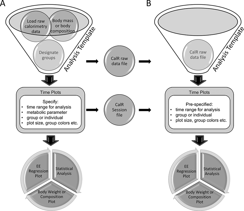
Users will select an analysis template that best matches their experimental design.

A) First-time analysis of an experiment includes loading raw indirect calorimetry data, optionally loading body composition data, and assigning animals into groups. This raw data can be exported into a standardized CalR data file for fast loading in subsequent sessions. Plotting parameters including the time range for analysis and other aesthetic preferences are set and visualized. These settings are saved as a CalR Session file. Once parameters are defined, statistical analysis and additional plotting results are available. B) Exported CalR raw data files and CalR Session files allow fast, transparent analysis and a record for reproducible research. Simply stated, the CalR data file is an unaltered experimental record. The CalR session file contains what was done to produce the analysis.

Defining an experiment.

Each indirect calorimetry run may contain more than one experimental intervention. We present an example in which mice are maintained at thermoneutrality (30°C) for three days followed by a transition to 4°C, (Figure 2). The time corresponding to the experimental period of interest can be selected with a slider bar under the “Time Plots” tab (see Supplemental Materials). A “Notes” section is included to allow the user to describe the criteria used in selecting the interval used for analysis. In providing a generalized framework for analysis, this single experiment analysis offers the greatest flexibility for a range of experimental designs.

Figure 2. Defining an experiment.

This one calorimetry run included two experiments in which two groups of mice were maintained at thermoneutrality (30°C) (Experiment 1) followed by a transition to a cold challenge and maintenance at 4°C (Experiment 2). Users of CalR would sequentially analyze these two experiments by selecting the corresponding time regions.

Analysis and experiment templates.

CalR provides the flexibility to interpret many common experimental designs. Each indirect calorimetry experiment is unique, but we have created standardized templates for many common practices (Figure 3). Users are directed to select a template which will apply the most suitable statistical approach. For this reason, we have prepared templates to analyze the following seven commonly encountered experimental designs and one template to combine experimental runs from different times on different subjects. A description of each template including a sample data set and step-by-step instructions are included (Supplemental Materials):

1. Two groups (e.g., two distinct genotypes). A common paradigm where two groups are studied simultaneously for more than 12 hours (Supplemental Examples 1 and 2).

2. Two groups with acute treatment (e.g., administration of a beta-adrenergic receptor agonist to stimulate metabolism). This template is ideal for targeting analysis over a region of 12 hours or less. It includes time plots of metabolic differences from a designated start hour. Analysis is performed every hour (Supplemental Example 3).

3. Three ordered groups (e.g., dose-response or wildtype / heterozygous / knockout). This template is for observing dose effects, either allelic, pharmacologic or conditioning. Groups are ordered into a hierarchy for analysis, which includes post hoc tests (Supplemental Example 4).

4. Three factored group (e.g., Vehicle vs. two independent treatments or WT vs. two independent knockouts). Contrary to the ordered template, this does not assume a hierarchical ordering of the group variable. This makes the analysis, including post hoc tests, distinct from the previous template (Supplemental Example 5).

5. Four groups (e.g., two genotypes with two treatments, or four independent genotypes). This template allows for any combination of four independent comparators and includes post hoc tests (Supplemental Example 6).

6. Crossover experiment (for two groups and one intervention). The intervention regimen is alternating between two groups (e.g., vehicle followed by drug and drug followed by vehicle). Animals are examined for treatment effect, period effect, and interaction effect (treatment x period) (Supplemental Example 7).

7. Experimental run combination Tool. CalR also provides a template which generates a graphical interface to facilitate combining multiple experimental runs into one CalR data file (Supplemental Example 8).

Figure 3. Example data from five analysis templates.

Left column, Time Plot; Right column, Overall Experiment Summary.

A) Two-group template. VO₂ for two groups of mice monitored for four days at room temperature. B) Two-group acute response template. Food intake for two groups over ten hours following treatment. C) Three-group template: ordered. Body temperature in wildtype, heterozygote, and knockout animals maintained at 4°C. D) Three group template: non-ordered. Energy expenditure of wildtype and two independent knockout strains. E) Four-group template. Energy expenditure analysis of two genotypes of mice on two different diets. Not shown: Crossover template or run combination tool. Note: CalR plots are not normalized or adjusted to body weight, lean mass, or another allometric scaling.

Data visualization.

There are several tabs available in the CalR web pages for observing the data with distinct perspectives. Navigating the tabs, a user can see body mass and body composition bar plots, time plots, average value plots and regression plots. The data presented are not normalized by total body mass, lean body mass or any allometric scaling factor due to the significant distortions that these can introduce (Himms-Hagen, 1997). The values presented under the “Time Plots” tab are the mean values for each group per hour. In this tab, a caution button labeled “Abnormal Readings” may appear if any of the raw, non-excluded data points in the selected time are physiologically impossible (e.g., RER at 0.4). Clicking this button will display the qualifying criteria and the ID of the corresponding subject(s). Under the “Average Plots” tab, the mean value for each 24-hour, light, or dark photoperiods are presented, as well as overall means for the selected region of analysis. The experimental period of interest can be specified with a slider bar to perform analysis on one experiment at a time. Many of the features of the time plots can be customized using the dialog box to specify colors, sizes, or inclusion of error bars. Weight plots represent the mean body mass or body composition if these data are supplied. Regression plots are often informative for understanding the relationship between EE and mass, but require appropriate sample size for useful interpretation.

Transparency, portability, and reproducibility

The CalR Data file.

The data files produced by indirect calorimeters of different manufacturers are formatted differently. Nonetheless, data loaded into CalR from each of the three supported manufacturers are first transformed into a standardized format which can be exported as a CalR data file. The CalR data file contains the unmodified raw data for each animal as initially collected. As a complete standardized record of the experiment, a CalR data file can be shared or included as supplemental data.

The CalR Session file.

Outside of the raw calorimetry data, additional information is required to complete the analyses. This includes importing body weights or body compositions, designating groups, specifying which cages are to be included in the analysis, selecting the time of the experiment, and choosing aesthetic preferences. The session file allows for specific and reproducible analysis of either raw data or from a CalR file. Multiple CalR Session files should be produced for calorimetry runs with numerous distinct experiments. This modular format will considerably facilitate the sharing of information and the creation of repositories of metabolic data sets. We have included examples of generating and reading the CalR file in the vignettes included as Supplemental Materials.

The Excluded Data file.

As described above, CalR contains optional features to automatically remove outliers and manually exclude cages from the analyses. These specified data are neither plotted, included in the group averages nor included in statistical analyses. However, these data are retained within the CalR data file which is a complete record of the raw experimental data. Furthermore, manually selected cages and automatically identified outlier data are included together in an “excluded data” file accessible through the Time plots tab. When the “remove outlier” feature is toggled on, the investigator is strongly encouraged to review the downloadable excluded data file to confirm the validity of these exclusions.

Statistical approach

Overview.

CalR implements generalized linear models (GLM) to describe the group effect under investigation while properly accounting for body mass effects on mass-dependent metabolic variables, such as energy expenditure. For a selected time range, metabolic variable, and photoperiod, all of the data points that are not excluded are averaged into a single value per animal. This value will be used in the ANCOVA/GLM for each animal using the selected mass variable as the covariate. Alternatively, we tested the use of all measurements as individual data points with the use of a random effect variable to account for within-mouse correlation with no notable differences yielded between this and our current model. For measurements not associated with mass (e.g., respiratory exchange ratio), the difference between groups is analyzed by a one-way ANOVA (Figure 4A). To model mass-dependent variables, the body mass variable is specified by the user and included as a covariate. This action is required independently of whether or not the masses are significantly different between groups in order to better fit the data, (Allison et al., 1995; Arch et al., 2006; Kaiyala, 2014; Kaiyala et al., 2010; Kaiyala and Schwartz, 2011; Katch, 1972a; Katch, 1972b; Kronmal, 1993; Speakman et al., 2013; Tanner, 1949; Tschöp et al., 2012). However, one essential requirement for ANCOVA is that there is not a significant group by mass interaction. This means that it is reasonable to assume that the slope of EE on mass is the same for each group (i.e., the slopes of the groups must be parallel (Figure 4B)). How do we interpret an experiment in which the slopes are not parallel, groups have different associations between EE and mass, and the assumptions of ANCOVA have been violated? The GLM can adequately account for this scenario in what might unconventionally be called “ANOVA with interaction” or “ANCOVA for non-parallel slopes” (Kowalski et al., 1994) but is here referenced only as GLM for lack of more specific statistical nomenclature (Figure 4C). CalR will first perform a GLM; if a significant interaction effect is observed, the significance of the group, mass, and interaction effect are all reported. If there is no significant interaction effect, CalR returns an ANCOVA with group and mass effects only. This automated algorithm will prove applicable to most indirect calorimetry experiments. The two assumptions of this analysis are i) that a study animal’s measurements are independent of those from others and ii) the true distribution of the measurements within the population (e.g., mice of the same strain and genotype as the study animals) is approximately normally distributed.

Figure 4.

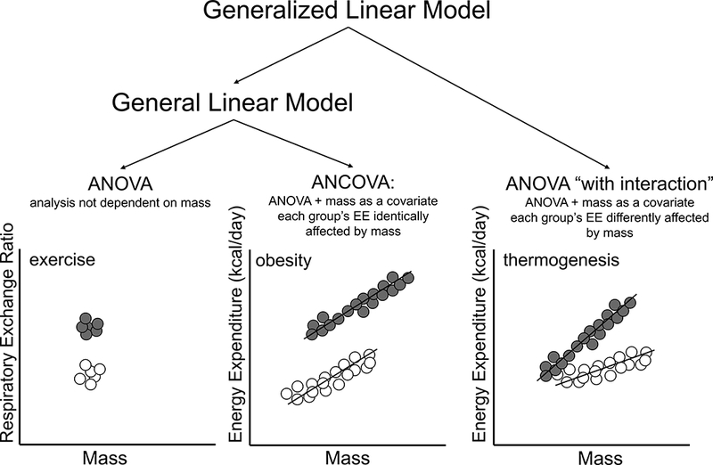
Analysis models of energy expenditure based on the general linear model. CalR determines the appropriate statistical model from the experimental data.

A) ANOVA is applied where mass or body composition is not expected to affect the metabolic parameter. A sedentary group (grey) compared to an exercised group (white) with similar mass would use the ANOVA to examine group differences in respiratory exchange ratio (RER). B) The ANCOVA (ANOVA with the addition of a covariate) when mass is significantly different, but slopes are parallel. This model could interpret an obese group of mice (gray) compared with lean controls (white) where greater mass and EE are observed. C) The GLM can interpret the different effect of mass on EE between groups by including an interaction effect. Mice with greater BAT mass (gray) with a more pronounced thermogenic response could be interpreted by this model.

ANOVA with interaction.

The GLM is performed on metabolic parameters that are anticipated to depend on body mass based on core physiological principles. From the group names listed in the “Input” tab, the first will be the reference group when this categorical variable is coded into the model. The GLM model contains ‘group’ as the main predictor variable, ‘mass’ as the covariate and the interaction between group and mass is included to test if it should be kept. The GLM performed in R is generalizable to:

➢ glm( y ~ mass + group + mass:group, family = gaussian( link = “identity” ))

Where y is a metabolic variable in the set of VO₂, VCO₂, EE, food intake, and water intake. For the “family” parameter we specify a Gaussian error structure, and for the “link” parameter we specify an identity link, which indicates that no transformations are to be made. The user selects mass to be total body mass, lean body mass, or fat mass. A type III model first computes the sum of squares, but if the interaction effect of group and mass is found to be insignificant, then it is dropped from the model.

ANCOVA.

When a mass-dependent parameter is estimated using the GLM and the interaction between group and mass is found to be insignificant, then the reduced GLM model resembles an ANCOVA model with the generalizable form:

➢ glm( y ~ mass + group, family = gaussian( link = “identity” ))

ANOVA.

The ANOVA is performed on parameters measured which are not strictly linked to body mass. The GLM model is reduced to an ANOVA with ‘group’ as the sole predictor variable and mass is not included in this model.

The ANOVA performed in R is generalizable to:

➢ glm( z ~ group, family = gaussian( link = “identity” ))

Where z is a metabolic variable in the set of respiratory exchange ratio (RER), locomotor activity, ambulatory activity, body temperature, and wheel running. These variables are independent of mass.

The analysis table of CalR is populated with the results of the ANCOVA or GLM computed with the covariate selected by the user (total mass, lean mass, or fat mass.) For each metabolic variable measured, CalR reports the effects of the group, mass, and interaction of mass and group (if significant). For this model to work, all of the included subjects must have their masses specified.

Post hoc.

For experiments with analysis of more than two groups, Tukey’s honest significant difference (HSD) post hoc test is performed and graphed to display confidence intervals. For the selected metabolic variable, the “Analysis” tab presents the mean difference with a 95% confidence interval for all pairwise group comparisons.

➢ glht( glm.model, mcp( group = “Tukey” ))

where glm.model is one of the aforementioned models depending on the metabolic parameter and whether or not the group by mass interaction effect is significant for mass-dependent parameters (i.e., ANOVA, ANCOVA, and ANOVA with interaction).

Automatic outlier detection.

Within the time range selected, the group means and standard deviations are calculated, stratified into 24-hour, light, and dark photoperiods. If “Yes” is selected for the “remove outlier” radio button, the values that fall beyond three standard deviations from the group mean for the respective light/dark period will be excluded from the analysis. Since VO₂, VCO₂, EE, and RER are interdependent, then the removal of data for one of these variables will lead to the removal of the data for all of them at the corresponding time point. Additionally, the indirect calorimetry apparatus is both complex and error-prone. Exclusion of data from malfunctioning feeders (e.g., momentary readings of negative food intake) is also justified. By default, automatic outlier detection is set to off, users must opt-in to remove these values from the analysis.

Manual subject exclusion.

After beginning a calorimetry run, animals may require veterinary intervention, or have reached a prespecified endpoint for humane euthanasia according to institutional guidelines. When one animal is physically removed from a cage, the data collected from this empty cage should cease to be included in the group analysis for the relevant experiment. Manual data exclusion is designed to remove all data from an empty cage starting at a designated time until the conclusion of the experiment. The “Subject Exclusion” tab is automatically populated with all subject names and the exclusion set to the hour at which the experiment concludes (i.e., no data excluded). While data from excluded cages will be omitted from the analysis, no data are removed or excluded from CalR data files. Next to each exclusion, there is an additional text box for the user to enter their reasoning for the corresponding exclusion. All excluded data, including user annotations from manual exclusions, are saved in an exportable data file and combined with automatic outliers, when in use.

Metabolic variables vs. time.

For visualization and analysis, the data read into CalR is cropped to the hour range selected by the user. To generate hourly time plots, CalR subsets the data by either group or subject, depending on user input, and computes averages and standard errors of the measurements at each hour for the metabolic variable being plotted. The values for the daily bar plots are calculated for each group at each photoperiod (light, dark, or 24-hour) and stratified by day, while the overall bar plot does not stratify by day. The structure of the data used for analysis consists of the average value of the metabolic variables for each subject for any one of the photoperiods.

Body masses and compositions.

CalR will automatically conduct unpaired two-sample t-tests on all two-group combinations to compute p-values that indicate if there are significant differences in the body mass averages of the groups.

➢ t.test( mass ~ group )

If in addition to total body mass, lean and fat masses are included, then CalR will also conduct similar statistical analyses of the body compositions. Bar plots display the average masses (and composition), and stars above the bars represent statistical significance. When more than two groups are involved, the significance tests are pairwise with the comparisons being indicated by the start and end location of the horizontal lines drawn above the bars.

Interactive 2D and 3D regression plots.

By default, CalR Regression plots display the average EE against total mass for the subjects included in the data. The default variable shown is EE because it is less prone to contain error than VO₂ and VCO₂ in open circuit indirect calorimeters (Arch et al., 2006). However, CalR provides the option to plot any of the following metabolic variables against body mass: VO₂, VCO₂, EE, RER, cumulative food intake, and body temperature. To examine the association between the metabolic variable and mass, we generate a plot with each subject’s mass against the average value of the selected metabolic variable of the respective subject over the experimental time frame chosen by the user (light, dark, 24-hour). Lines of best fit are produced for each group, with optional shading of the range of standard error. Slopes are then computed and compared by linear regression analysis. For the selected metabolic variable, time of day, and mass variable, CalR will automatically calculate the p-values of GLM-based coefficients to indicate if a significant group, mass or interaction effects exist. We also include the ability to plot EE vs locomotor activity, in which the activity effect on EE is reported in place of the mass effect. When lean mass and fat mass have been provided, the option to produce a three-dimensional plot of EE (or other metabolic variables) vs. lean and fat mass becomes available to the user. A plane of best fit, computed from a GLM that includes both lean mass and fat mass as covariates, is produced for each group. These 3D plots can be rotated, zoomed-in or saved as image files.

Data Analysis Example

CalR is foremost a tool to facilitate analysis of organismal energy balance experiments. Here we briefly describe one example of data analysis for an experiment of two groups with 12 wild-type and ten knockout mice. For a video of this example, see the two-minute Figure360 associated with this submission. Additional step-by-step instructions for this and other examples can be found in the Supplementary Materials. The user’s first step is to select and launch the two-group analysis template by navigating from the CalR home page to select “Templates”, and from the drop-down, selecting “Two groups”. Using the “Input” tab of the graphical user interface (Figure 5A) in the first column, raw data files or CalR data files are selected and uploaded. In the second column, we also wish to add body composition data by uploading a spreadsheet with animal identifiers, lean mass, fat mass, and total mass. In the third column, we assign group names and subject identifiers to the appropriate group. When the “Go to Plots” button is activated, the “Time Plots” tab is populated (Figure 5B). The default settings will plot oxygen consumption for the total duration of the experiment, averaged by group, with outliers removed. These and other settings can be adjusted by the user. A recommended practice is to exclude the initial 12–24 hour acclimation period of an experiment from the analysis (Tschöp et al., 2012). The “Generate Plot” button will populate hourly mean values in a time plot. In addition, daily mean values or overall averages will appear under the “Average Plots” tab. The bar plots are divided by photoperiod specified in the input tab (default light at 0700 and default dark at 1900 hours). Error bars are standard error of the mean (SEM). These data are plotted without normalization or adjustment to mass. In the “Regression Plots” tab (Figure 5C) we plot metabolic variables vs. either one or two mass parameters (lean, fat or total). At the bottom of the plot are values from the analysis of whether the selected variable is affected by mass, group, or interaction. Under standard room-temperature housing and experimental conditions, we expect a significant mass effect (p<0.05), where greater body mass will correlate to greater metabolic variables including VO₂, VCO₂, EE, and Food Intake. This information can be valuable for understanding the quality of the experimental conditions. As such, an alert will be displayed if either the mass effect is not significant or a mass by group interaction effect is present. While these results can be visualized with each metabolic parameter in the regression plots tab, a full table of results is available under the Analysis Tab (Figure 5D). See Vignettes in Supplementary Materials for additional examples. Other features of note, the data being visualized (time range selected, groups specified, outliers removed) can be exported for further analysis as CalR data files and CalR session files.

Figure 5.

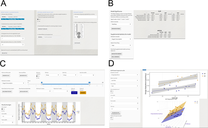
Example of the CalR graphical user interface for the two-group analysis.

A) Input tab for data upload and group assignments. B) Time Plots tab for data visualization of individual metabolic parameters for the selected period. Selected plots for oxygen consumption vs time. Shading denotes dark and light photoperiod. C) Results of statistical tests are shown in the “Analysis tab”. D) Regression Plots tab allows for analysis of metabolic data vs. mass in two or three dimensions EE vs LBM and/or FM.

Discussion

CalR provides users with much-needed comprehensive data analysis tools for indirect calorimetry experiments. Using CalR will enable easy access to analyze data using the GLM, which should reduce the “recurring problem” where EE is inappropriately normalized by allometric scaling or divided by lean body mass in mice of different body compositions (Arch et al., 2006; Butler and Kozak, 2010). Indeed, CalR removes much of the guesswork facing investigators who are understandably more interested in biological interpretation and less focused on learning specialized statistical methods. Rigorous hypothesis testing requires formally defining the model and parameters prior to analysis. We implement a defined computational and statistical procedure, tackling and obviating the pressing issues that accompany the time-demanding, highly variable, and otherwise virtually untraceable steps typically taken towards generating complete analyses.

ANCOVA has been the method of choice for indirect calorimetry experiments as it efficiently models the effect of mass on multiple metabolic variables. However, by definition, the ANCOVA cannot analyze a differential interaction between mass and group on EE (Figure 4). One approach to circumvent these limitations is using the Johnson-Neyman procedure (D’Alonzo, 2004) to find and analyze regions where there is no significant interaction between groups. While the Johnson-Neyman procedure permits the ANCOVA to be performed, it is accompanied by the dual drawbacks of i) excluding data which decreases already limited statistical power and ii) possibly compromises interpretations in cases where the interaction effect may be biologically relevant. Although ANCOVA has been widely recognized as a suitable model for indirect calorimetry data analysis, it is essential to have the data drive the decision on which models to use. By transitioning from classical linear regression (ANOVA or ANCOVA) to GLM, assumptions of normality and constancy of variance within the samples being tested are no longer required (McCullagh and Nelder, 1998). In the GLMs, interaction effects are included when they are statistically significant. Since the interaction effect could be an essential component of an experimental metabolic story, it is added in CalR to provide a more complete and applicable analysis.

CalR will allow for the sharing of raw data files of experiments across calorimetry platforms. This will enable whole body physiology to join the broader trend in biomedical research led by genomics and transcriptomics. The ability to efficiently share files as supplemental data will foster increased transparency and reproducibility with the cooperation of interested investigators. We propose a centralized repository of CalR indirect calorimetry data files to accelerate global research into metabolism and whole-body physiology.

Despite its many existing features, CalR is designed to support further innovation. Specifically, newer calorimetry systems provide more frequent sampling times and higher-resolution understanding of metabolic parameters. However, this nuance is lost in ANOVA/ANCOVA/GLM analyses. Regardless of the high-resolution time data, the consensus approach of ANCOVA-like analysis depends upon a single mean value per metabolic variable per mouse (Kaiyala; Speakman et al., 2013; Tschöp et al., 2012). Future advances may be possible by implementing time series and body composition into a statistical framework for indirect calorimetry. CalR opens the door for a dialogue on how indirect calorimetry data should best be analyzed under different experimental conditions. What CalR offers investigators is the architecture for ensuring that their indirect calorimetry data are properly handled and analyses are conducted in a transparent and reproducible manner.

Limitations

There are notable caveats to consider with implementing CalR for analysis. Good experimental design is critical for reproducible analysis. Small sample size or short run times may compromise experimental interpretation due to large individual animal variation. We recommend guidelines for experimental design for indirect calorimetry experiments (Tschöp et al., 2012). CalR cannot detect if a calorimeter is out of calibration and may, therefore, return results which are predicated on faulty data. As with any experimental system, quality control is dependent on the rigorous upkeep of the instrument and vigilance of the operator. Even under optimal conditions, animals may become sick, or equipment failure can spoil the appearance of an experiment. CalR provides tools which will allow for the exclusion of data from cages where animals have been removed from an experiment for humane reasons. CalR also provides the ability to combine multiple experimental runs to help overcome the difficulties in generating sufficient numbers of sex-and age-matched littermates for the study of genetically modified mouse lines. The investigator is responsible for justifying the appropriateness of two groups being joined for analysis, as CalR cannot. Another important consideration is to look beyond the p-values for interpretation of the results. Just as, if not more, importantly is the effect size between the groups and physiological relevance of the result. Since sample size is highly influential on the ability to detect a true difference, and it is often challenging to have a large sample size for these types of experiments (Kaiyala, 2014), it would be unreasonable to discard (or fail to publish) results that are not statistically significant but show potentially biologically important effect sizes (Gelman and Stern, 2006).

KEY RESOURCES TABLE

REAGENT or RESOURCE	SOURCE	IDENTIFIER
Software and Algorithms
CalR	This paper	OMICtools: OMICS 23756 RRID:SCR_015849 https://www.CalRapp.org

STAR Methods

Contact for resource sharing

Further information and should be directed to and will be fulfilled by the Lead Contact, Alexander Banks (abanks@bwh.harvard.edu)

Experimental Model and Subject Details

Eight examples are included in the Methods S1 File. The subject details for the mice in these studies are described below. All animal experiments were approved by the Institutional Animal Care and Use Committee (IACUC) of the Harvard Center for Comparative Medicine (HMS), the Brigham and Women’s Hospital (BWH), or Vanderbilt University. Some of the data sets were artificially contrived to illustrate specific aspect of CalR, while others are presented as collected. These are indicated below.

Examples 1 and 2 are idealized synthetic data sets meant to illustrate two groups of mice with and without an interaction effect between mass and all mass-dependent metabolic variables.

Example # and Description	Genetic Background	Sex	Age (wk, approx.)	Diet	IACUC Approval
1. Two-group ANCOVA
2. Two-group interaction
3. Two-group acute response	C57Bl/6	M	20	60% HFD	BWH
4. Three-group (ordered)	C57Bl/6 × 129S/v mixed	M	16	Standard Chow Picolab 5053	HMS
5. Three-group (unordered/factorial)	C57Bl/6	M	16	Standard Chow Picolab 5053	BWH
6. Four-group	C57Bl/6	M	20	Standard Chow and 60% HFD	BWH
7. Combining Runs	C57Bl/6	M	14	Standard Chow Picolab 5053	HMS
8. Two-group crossover design	C57Bl/6	M	15	Standard Chow Picolab 5053	Vanderbilt

Method Details

The experimental parameters for each of the eight example data sets are indicated below.

Example # and Description	Equipment	Ambient temperatures	Data Described in Methods S1
1. Two-group ANCOVA		Room temp	After acclimation
2. Two-group interaction		Room temp	After acclimation
3. Two-group acute response	CLAMS	22C→30C→CL	CL injection
4. Three-group (ordered)	CLAMS	30C→22C→ 4C→22C	4C
5. Three-group (unordered/factorial)	CLAMS	30C→4C	30C→ 4C
6. Four-group	CLAMS	22C→30C→CL	22C
7. Combining Runs	CLAMS	23C	23C
8. Two-group crossover design	Prometheon	23C	23C

*CL, beta-3 adrenergic agonist CL-316,243

DATA and SOFTWARE AVAILABILITY

Example data sets 1–8 can be found in Methods S1 CalR can be accessed at https://CalRapp.org

Highlights.

• CalR is a free web tool for analysis of experiments using indirect calorimetry

• Imports data, generates plots, and determines the best-fit statistical model

• Outputs a standardized CalR file which can be shared, deposited and re-read by CalR

• Increases speed, transparency and reproducibility of energy balance experiments

References

- Allison D, Paultre F, Goran M, Poehlman E, and Heymsfield S (1995). Statistical considerations regarding the use of ratios to adjust data. International journal of obesity and related metabolic disorders: journal of the International Association for the Study of Obesity 19, 644–652. [PubMed] [Google Scholar]
- Arch J, Hislop D, Wang S, and Speakman J (2006). Some mathematical and technical issues in the measurement and interpretation of open-circuit indirect calorimetry in small animals. International journal of obesity 30, 1322–1331. [DOI] [PubMed] [Google Scholar]
- Betz MJ, and Enerback S (2017). Targeting thermogenesis in brown fat and muscle to treat obesity and metabolic disease. Nat Rev Endocrinol advance online publication. [DOI] [PubMed] [Google Scholar]
- Butler AA, and Kozak LP (2010). A Recurring Problem With the Analysis of Energy Expenditure in Genetic Models Expressing Lean and Obese Phenotypes. Diabetes 59, 323–329. [DOI] [PMC free article] [PubMed] [Google Scholar]
- Calle EE, Rodriguez C, Walker-Thurmond K, and Thun MJ (2003). Overweight, obesity, and mortality from cancer in a prospectively studied cohort of U.S. adults. N Engl J Med 348, 1625–1638. [DOI] [PubMed] [Google Scholar]
- D’Alonzo KT (2004). The Johnson-Neyman Procedure as an Alternative to ANCOVA(). Western journal of nursing research 26, 804–812. [DOI] [PMC free article] [PubMed] [Google Scholar]
- Drucker Daniel J. (2016). Never Waste a Good Crisis: Confronting Reproducibility in Translational Research. Cell metabolism 24, 348–360. [DOI] [PubMed] [Google Scholar]
- Fisher RA (1947). The analysis of covariance method for the relation between a part and the whole. Biometrics 3, 65–68. [PubMed] [Google Scholar]
- Flier JS (2017). Irreproducibility of published bioscience research: Diagnosis, pathogenesis and therapy. Molecular metabolism 6, 2–9. [DOI] [PMC free article] [PubMed] [Google Scholar]
- Gelman A, and Stern H (2006). The Difference Between “Significant” and “Not Significant” is not Itself Statistically Significant. The American Statistician 60, 328–331. [Google Scholar]
- Guyenet SJ, and Schwartz MW (2012). Regulation of food intake, energy balance, and body fat mass: implications for the pathogenesis and treatment of obesity. The Journal of Clinical Endocrinology & Metabolism 97, 745–755. [DOI] [PMC free article] [PubMed] [Google Scholar]
- Himms-Hagen J (1997). On Raising Energy Expenditure in ob/ob Mice. Science 276, 1132. [DOI] [PubMed] [Google Scholar]
- Jarvis MF, and Williams M (2016). Irreproducibility in Preclinical Biomedical Research: Perceptions, Uncertainties, and Knowledge Gaps. Trends Pharmacol Sci 37, 290–302. [DOI] [PubMed] [Google Scholar]
- Kaiyala KJ MMPC Energy Expenditure Analysis Page.
- Kaiyala KJ (2014). Mathematical model for the contribution of individual organs to non-zero y-intercepts in single and multi-compartment linear models of whole-body energy expenditure. PloS one 9, e103301. [DOI] [PMC free article] [PubMed] [Google Scholar]
- Kaiyala KJ, Morton GJ, Leroux BG, Ogimoto K, Wisse B, and Schwartz MW (2010). Identification of body fat mass as a major determinant of metabolic rate in mice. Diabetes 59, 1657–1666. [DOI] [PMC free article] [PubMed] [Google Scholar]
- Kaiyala KJ, and Schwartz MW (2011). Toward a more complete (and less controversial) understanding of energy expenditure and its role in obesity pathogenesis. Diabetes 60, 17–23. [DOI] [PMC free article] [PubMed] [Google Scholar]
- Katch V (1972a). Correlational υ Ratio Adjustments of Body Weight in Exercise-Oxygen Studies. Ergonomics 15, 671–680. [DOI] [PubMed] [Google Scholar]
- Katch VL (1972b). Use of the oxygen-body weight ratio in correlational analyses: spurious correlations and statistical considerations. Medicine and science in sports 5, 253–257. [PubMed] [Google Scholar]
- Kowalski CJ, Schneiderman ED, and Willis SM (1994) ANCOVA for nonparallel slopes: the Johnson-Neyman technique. International journal of bio-medical computing 37, 273–286. [DOI] [PubMed] [Google Scholar]
- Kronmal RA (1993). Spurious correlation and the fallacy of the ratio standard revisited. Journal of the Royal Statistical Society. Series A (Statistics in Society), 379–392. [Google Scholar]
- McCullagh P, and Nelder JA (1998). Generalized linear models. (Boca Raton: Chapman & Hall/CRC; ). [Google Scholar]
- Pelleymounter M, Cullen M, Baker M, Hecht R, Winters D, Boone T, and Collins F (1995). Effects of the obese gene product on body weight regulation in ob/ob mice. Science 269, 540–543. [DOI] [PubMed] [Google Scholar]
- R Core Team (2017). R: A language and environment for statistical computing. (Vienna, Austria: R Foundation for Statistical Computing; ). [Google Scholar]
- Speakman JR, Fletcher Q, and Vaanholt L (2013). The ‘39 steps’: an algorithm for performing statistical analysis of data on energy intake and expenditure. Disease models & mechanisms 6, 293–301. [DOI] [PMC free article] [PubMed] [Google Scholar]
- Stanford KI, Middelbeek RJ, Townsend KL, An D, Nygaard EB, Hitchcox KM, Markan KR, Nakano K, Hirshman MF, Tseng YH, et al. (2013). Brown adipose tissue regulates glucose homeostasis and insulin sensitivity. J Clin Invest 123, 215–223. [DOI] [PMC free article] [PubMed] [Google Scholar]
- Tanner J (1949). Fallacy of per-weight and per-surface area standards, and their relation to spurious correlation. Journal of applied physiology 2, 1–15. [DOI] [PubMed] [Google Scholar]
- Tschöp MH, Speakman JR, Arch JR, Auwerx J, Brüning JC, Chan L, Eckel RH, Farese RV Jr, Galgani JE, and Hambly C (2012). A guide to analysis of mouse energy metabolism. Nature methods 9, 57–63. [DOI] [PMC free article] [PubMed] [Google Scholar]
Associated Data
This section collects any data citations, data availability statements, or supplementary materials included in this article.