BREAST CANCER HISTOPATHOLOGY IMAGE ANALYSIS PIPELINE FOR TUMOR PURITY ESTIMATION

Abstract

The translation of genomic sequencing technology to the clinic has greatly advanced personalized medicine. However, the presence of normal cells in tumors is a confounding factor in genome sequence analysis. Tumor purity, or the percentage of cancerous cells in whole tissue section, is a correction factor that can be used to improve the clinical utility of genomic sequencing. Currently, tumor purity is estimated visually by expert pathologists; however, it has been shown that there exist vast inter-observer discrepancies in tumor purity scoring. In this paper, we propose a quantitative image analysis pipeline for tumor purity estimation and provide a systematic comparison between pathologists’ scores and our image-based tumor purity estimation.

1. INTRODUCTION

Genomic sequencing is an established tool in basic research, and the advent of massively-parallel next-generation sequencing (NGS) has allowed the adoption of genomic sequencing as a clinical diagnostic tool. However, existing challenges in the analysis of NGS data serve to limit its clinical utility. One of these challenges is the infiltration of non-cancerous cells in tumors, which affects the interpretation and clinical utility of genomic analyses. For this reason, the estimation of tumor purity (TP) has been an important topic of many studies to compensate for the effect of non-cancerous cells [1][2][3].

Currently, tumor purity scores are often derived from the visual estimation of tumor specimens by trained pathologists. However, it has been shown that there exist vast inter-observer discrepancies in the estimation of TP by pathologists [4], which may lead to incorrect indicators of prognosis and/or response to treatment in certain cancer types. For example, TP can indicate the presence of clonal populations of cancerous cells in a given tumor, a feature that may help predict prognosis and response to treatment [5][6][7]. Another confounding effect caused by differences in TP [8] across tumors is the detection of DNA copy number variations (CNV), a feature which has been shown to contribute to cancer pathogenesis [9][10][11]. Thus, an accurate and consistent estimation of TP promises to be a useful measure, not only to enhance the utility of genomic sequencing data, but also for better clinical outcome.

Recently, many statistical algorithms have been developed in an attempt to measure TP from DNA expression data [1]. However, these methods heavily rely on statistical assumptions and thus can not be generalized to many forms of sequencing data [2]. Furthermore, these methods do not identify whether a mutation is occurring in a subpopulation of cells, an occurrence that can have significant implications. For these reasons, it is advantageous to estimate TP directly from quantitative image analysis.

In [3], the authors proposed a method to measure TP based on quantitative analysis of hematoxylin and eosin (H&E)-stained images of tumor specimens. To do this, they acquired manual annotations by pathologists and used a support vector machine classifier to classify individual nuclei into four different classes (cancer, lymphocyte, stromal, and artifacts), achieving a classification accuracy of 90.1%. They showed that image-based TP estimation is correlated with pathologists’ TP scores and demonstrated that quantitative image analysis is useful for improving survival prediction by refining and complementing genomic analysis. However, correlation comparisons may not be enough to decide clinical accuracy, and furthermore, inherent challenges in image analysis such as nuclei detection rate, segmentation accuracy, or imperfect classification rate, which could cause bias in image-based TP estimation, were not explored further.

In this paper, we develop a quantitative image analysis pipeline that includes annotation, segmentation and classification. We also introduce a method to provide a systematic comparison between pathologists’ TP and image-based TP estimations. We envision that this framework will allow us to have a better understanding of TP estimation based on quantitative image analysis.

2. QUANTITATIVE IMAGE ANALYSIS PIPELINE

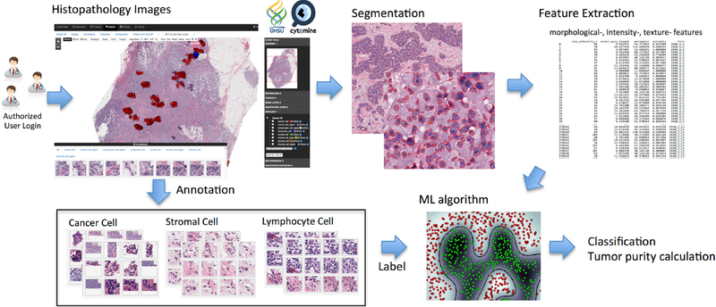
Figure 1 shows a conceptual illustration of the proposed pipeline. In the following section, we will explain each module in detail.

Fig. 1.

Conceptual illustration of the proposed pipeline: histopathology image annotation, segmentation, feature extraction, classification and tumor purity calculation.

2.1. Annotation tool

In order to collect annotated data from tumor specimens, we installed Cytomine [12], an open-source software designed for image-based collaborative studies, on a campus-wide server. H&E whole-slide images (WSI, 20 × magnification) of breast cancer tumor specimens obtained and processed at OHSU using the same protocol were uploaded to Cytomine, and annotations were performed by pathologists using Cytomine’s web user-interface to annotate individual as well as large regions of nuclei. Annotations and their respective image coordinates were downloaded using Cytomine’s Python client. Combined with our segmentation results (section 2.2), individual nuclei were then categorized into “cancer”, “stromal”, “lymphocyte” and “normal” classes, resulting in a total of 27,863 labeled cancer nuclei and 4,831 non-cancerous nuclei for 10 WSI samples. A subset of 4,831 cancer nuclei was randomly selected in order to balance the data for a total of 9,662 labeled nuclei across the 10 WSI images.

2.2. Segmentation

In this paper, we used our automatic nuclei segmentation algorithm [13]. In H&E stained section, hematoxylin stains cell nuclei blue while eosin stains other structures in various shades of red and pink. Since each pixel has a specific intensity and also represents a part of morphological features, by mapping each pixel with useful morphological features and grouping neighboring pixels with similar features, one can differentiate between foreground and background, or between different tissues and nuclei. Thus, nuclei segmentation can be effectively performed by partitioned groups. More detailed information can be found in [13].

2.3. Training Data Set

Since we have obtained labelled data from pathologists’ annotations and individual nuclei masks from the segmentation results, we constructed the training data sets for supervised machine learning. Because we are interested in tumor purity estimation, segmented nuclei are simply classified into “cancerous” and “non-cancerous” categories based on the pathologists’ annotations; thus we merged stromal, lymphocyte and normal nuclei into the “non-cancerous” nuclei class.

2.4. Classification

In order to classify segmented nuclei as cancerous or non-cancerous, we used supervised classification techniques. First, we used a balanced training data set (as described in section 2.1) and trained an L1-regularized logistic regression (LR) classifier with basic features including intensity and morphology features (area, perimeter, shape indexes, etc.) extracted from 9,662 labeled cells. We used 90% of the data for training our classifier and held out 10% of the data as a testing set. In order to measure the performance of the classifier on unseen data, we used 10-fold cross-validation, in which for each “fold”, a classifier is trained using 90% of the training data and the model is validated on 10% of the training data. The performance was then calculated as the prediction accuracy on our testing set. Using only intensity and morphology features, we obtained 79.0% prediction accuracy using the above process.

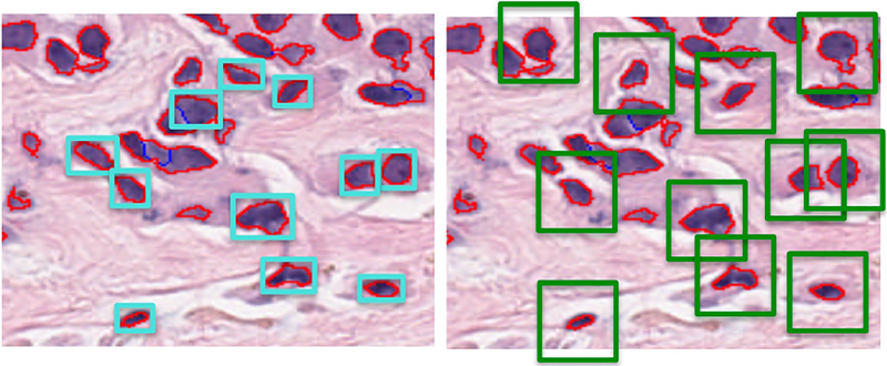
To improve the performance of the classifier, we added texture features extracted from each segmented nuclei mask and trained our classifier again. In order to calculate texture features, we calculated a gray-level co-occurrence matrix (GLCM) based on a patch determined by the bounding box of each individual nuclei as shown in Figure 2 (left), where patch size depends on the size of segmented nuclei; a GLCM describes the second order statistics of pixel pairs located at a given offset. Haralick texture features for each color channel, including contrast, dissimilarity, homogeneity, energy, correlation and angular second moment (ASM) are then calculated based on each nucleus’s GLCM. We obtained 82.0% prediction accuracy using our testing set.

Fig. 2.

Image patch for texture feature extraction where red boundaries represent individual segmented nuclei and blue boundaries represent separation of touching nuclei using watershed algorithm: (left) initial patch for texture feature extraction based on the bounding box of segmented nuclei; (right) fixed size patch centered at centroids of segmented nuclei allows for context-specific feature extraction and increases classification accuracy.

In order to extract context-specific texture features, we chose a fixed patch size of 64 × 64 pixels per individual nucleus as shown in Figure 2 (right). This allowed us to include information about the individual nucleus’ environment such as features related to neighboring nuclei and their density. This is inspired by deep learning architecture for feature learning where some of the input features may include neighboring nuclei information. Following this adjustment in texture feature extraction, we obtained 94.5% classification accuracy using our testing set.

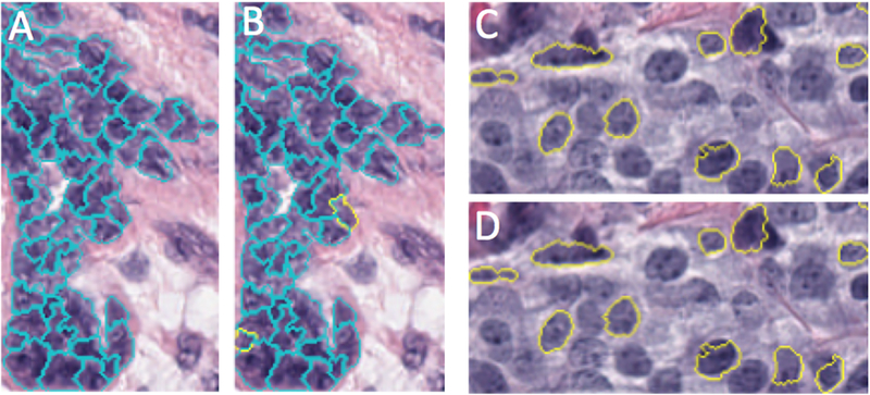
Finally, we also trained a support vector machine (SVM) [14] using the radial basis function kernel with the same features. All prediction results are summarized in Table 1. Each model we used has parameters that affect the accuracy; in order to achieve maximal training and cross-validation accuracy, we performed a single parameter grid search in which one parameter is calibrated while the others are held at default values and the model is trained. Using this method we obtained 98.4% prediction accuracy for the training data set. Once the best parameters were determined, we checked for overfitting by testing the model on a testing set and obtained similar precision accuracy (98.6%). A confusion matrix is shown in Table 2 for this testing data set, and Figure 3 shows the comparison between the ground truth (pathologists’ annotation) and our prediction (sampled ROI).

Table 1.

Classification results of different classifiers/features (¹: with basic features, ²: with basic + texture features, and ³: with basic + texture features with fixed patch).

Classifier	Prediction	Sensitivity	Specificity
LR1	0.79	0.80	0.78
LR2	0.82	0.84	0.80
LR3	0.95	0.93	0.96
SVM3	0.99	0.98	0.99

Table 2.

Confusion matrix (testing data set).

		True diagnosis
		cancer	non-cancer
Prediction	cancer	479	10
	non-cancer	4	473

Fig. 3.

Example of a prediction result from a test data set: (A and C) Nuclei that have been annotated with pathologists’ labels overlaid on top of our nuclei segmentation. (B and D) Classes predicted by our SVM classifier for annotated nuclei. Cancerous nuclei outlined in yellow, non-cancerous nuclei outlined in cyan. (Lack of outlines for some nuclei represent nuclei without pathologists’ annotations).

3. RESULT AND DISCUSSION

We define tumor purity (TP_#) as follows:

$${\text{TP}}_{\text{\#}}=\frac{n_T}{n_T+n_N}=\frac{1}{1+\text{\hspace{0.17em}γ}}$$ (1)

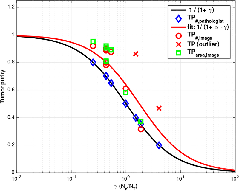
where n_T represents the number of tumor cells, n_N represents the number of normal cells and we denote the ratio of these numbers by γ ≜ n_N/n_T. For example, if we have three times more normal cells than tumor cells (i.e., γ = 3), then we have TP_#=0.25. In Figure 4, solid black line shows a nonlinear relationship between γ and TP based on (1) and blue diamond marker represents pathologists’ tumor purity score across 10 WSI samples where γ is simply calculated based on (1), i.e., $\text{γ\hspace{0.17em}=\hspace{0.17em}}\frac{1-{\text{TP}}_{\#}}{{\text{TP}}_{\#}}.$ Note that we use semi-log plot (i.e., x-axis is plotted on a logarithmic scale).

Fig. 4.

Tumor purity comparison where α = 0.5688 with 95% confidence bounds.

With this notion, you can see how TP changes according to γ. For example, if TP changes from 0.8 to 0.4 (reduced by half), γ changes from 0.25 to 1.5 (increased by 6 times). Thus, when pathologists examine two different WSI samples which have tumor purity 0.8 and 0.4 respectively, they should see the difference from 0.25 and 1.5 in γ. Similarly, if TP changes from 0.8 to 0.2 (reduced by one-quarter), γ changes from 0.25 to 4 (increased by 16 times). This numerical example illustrates that sensitivity factor of pathologists evaluation may vary over the ranges of γ.

Red circle marker in Figure 4 represents tumor purity estimations from quantitative image analysis showing that our image-based TP estimations are correlated with pathologists’ score but overall, our estimation is slightly higher than pathologist’s score (note that the red cross marker represents outliers, where the WSI includes artifacts, such as tissue folds and bubbles). There could be many possible reasons for this overestimation, such as over-segmentation, overall detection rate, pathologists’ bias, etc. In terms of over-segmentation, for example, cancer cells are clustered together in general so we need to use watershed algorithm to separate the clustered cells as shown in Figure 3. However, normal cells such as lymphocytes are not clustered (i.e., not touching each other) so they can be segmented well without any separation. Then, γ could be smaller than the ground truth (thus, higher TP estimation) because we may have more chance to do over-segmentation in tumor cell regions.

In order to provide a systematic comparison between pathologists’ scores and our TP estimation, we fit our TP_# score with given γ calculated from pathologists’ TP score to understand this discrepancy. Our fitting function shows ${\text{TP}}_{\#}=\frac{1}{1+0.5688\cdot \text{\hspace{0.17em}γ}}$ where 1.7581(=1/0.5688) could be the scaling factor reflecting this over-segmentation. There could be another possibility, for example, pathological scores may reflect primarily the area ratio:

$${\text{TP}}_{area}=\frac{A_T}{A_T+A_N}=\frac{1}{1+\frac{A_N}{A_T}}=\frac{1}{1+\frac{{ā}_N\cdot n_N}{{ā}_T\cdot n_T}}=\frac{1}{1+\beta \cdot \text{\hspace{0.17em}γ}}$$ (2)

where A_T , A_N represent total area covered by tumor and normal cell in tissue section respectively, ${ā}_T,{ā}_N$ represent mean area size of tumor and normal cell respectively and $\beta ={ā}_N/{ā}_T$ reflects the ratio of these numbers. Without loss of generality, we have TP_# ≤ TP_area as shown in Figure 4 where TP_{area, image} (green square) is slightly higher than TP_#,image (red circle). Note that equality holds when mean of tumor cell area size is equal to mean of normal cell area size, i.e., ${ā}_n={ā}_T$. With this notion (i.e., pathologist scores reflect primarily the area of tumor cells seen in a given area), we need to compensate $\text{γ}\left(=\frac{1}{\beta }\cdot \frac{1-{\text{TP}}_{area}}{{\text{TP}}_{area}}\right)$ since tumor cell size is bigger than normal cell size (${ā}_N\le {ā}_T,$ i.e.,β ≤ 1) in general.

4. CONCLUSION

In this paper, we developed a quantitative image analysis pipeline for tumor purity estimation. We demonstrated that our TP estimations are correlated with, but slightly higher than the estimates from pathologists. To understand inherent challenges in image analysis for improved clinical accuracy, we introduced a simple but effective way to provide a systematic comparison. To better understand this small discrepancy and the statistical comparison, we are currently applying our image analysis pipelines on larger data sets.