Combination of rs-fMRI and sMRI Data to Discriminate Autism Spectrum Disorders in Young Children Using Deep Belief Network

Abstract

In recent years, the use of advanced magnetic resonance (MR) imaging methods such as functional magnetic resonance imaging (fMRI) and structural magnetic resonance imaging (sMRI) has recorded a great increase in neuropsychiatric disorders. Deep learning is a branch of machine learning that is increasingly being used for applications of medical image analysis such as computer-aided diagnosis. In a bid to classify and represent learning tasks, this study utilized one of the most powerful deep learning algorithms (deep belief network (DBN)) for the combination of data from Autism Brain Imaging Data Exchange I and II (ABIDE I and ABIDE II) datasets. The DBN was employed so as to focus on the combination of resting-state fMRI (rs-fMRI), gray matter (GM), and white matter (WM) data. This was done based on the brain regions that were defined using the automated anatomical labeling (AAL), in order to classify autism spectrum disorders (ASDs) from typical controls (TCs). Since the diagnosis of ASD is much more effective at an early age, only 185 individuals (116 ASD and 69 TC) ranging in age from 5 to 10 years were included in this analysis. In contrast, the proposed method is used to exploit the latent or abstract high-level features inside rs-fMRI and sMRI data while the old methods consider only the simple low-level features extracted from neuroimages. Moreover, combining multiple data types and increasing the depth of DBN can improve classification accuracy. In this study, the best combination comprised rs-fMRI, GM, and WM for DBN of depth 3 with 65.56% accuracy (sensitivity = 84%, specificity = 32.96%, F1 score = 74.76%) obtained via 10-fold cross-validation. This result outperforms previously presented methods on ABIDE I dataset.

Introduction

In 1 of every 150 children, autism spectrum disorders (ASDs) which are regarded as relatively common neurodevelopmental conditions are presented [1, 2]. Statistics show that the risk of ASD is increasing in the world. The present data from the US Department of Education [3] showed that the risk of autism is increasing by 10 to 17% annually. As a developmental disorder, ASD has a widespread effect which manifests in social communications, social skills, imagination, and behavior [4–9]. In most cases, this disorder is only diagnosed when symptoms have erupted and the patient is suffering from untreatable complications. Therefore, correct diagnosis of ASD in the early stages is considered very important.

In the treatment of ASD, early diagnosis is the most important factor. The most important factor in treating ASD is early diagnosis. In cases of unclear behavioral symptoms, biomarkers are needed to improve diagnostic precision. It is also required for the identification of infants and young children at risk of ASD, prior to the manifestation of reliable behavioral symptoms [10, 11]. The introduction of new imaging methods, such as functional and structural magnetic resonance imaging (fMRI and sMRI), offers a more constructive approach to early diagnosis of neurological brain disorders. According to Mueller et al. [12], neurobiological correlations for brain architecture and function were detected by these methods. In addition, for better diagnosis, these methods could be used to detect potential early markers of the disease.

In recent years, magnetic resonance (MR) images were used to identify patients with autism. Several studies have been conducted using MRI techniques to diagnose ASD based on resting-state functional magnetic resonance imaging (rs-fMRI) [11, 13–17], gray matter (GM) [18, 19], and white matter (WM) [19, 20]. With these recent advances, it is still not clear if these structural and functional abnormalities are enough to differentiate ASD from typical control (TC) individuals. The combination of function and structure could provide more information about altered brain patterns and connectivity [21–24]. Studies are yet to be conducted which will combine rs-fMRI with two other different types of matters for sMRI data (GM and WM).

The use of machine learning algorithms in medical diagnosis has been increasing gradually. In the field of medical imaging which includes computer-aided diagnosis, machine learning plays an important role. In a bid to improve diagnostic performance, researchers are now using modern machine learning methods like deep learning. This method is employed for exploitation of the high-level latent and complicated features in data [25–31], to solve medical imaging-related problems. The initial incentive of this field is inspired by an examination of the neural structure of the brain where nerve cells make perception possible by sending messages to each other [32]. Based on different assumptions on how these cells connect, different models and structures have been proposed; however, these models do not naturally exist in the human brain, because the human brain is more complex. A lot of interests have been raised consequent upon the successful application of greedy layer-wise training using restricted Boltzmann machine (RBM), deep belief network (DBN), one of the deep learning methods and a generative probabilistic model [33–35]. Recently, there have been breakthroughs in medical imaging analysis which is as a result of DBN usage.

This paper introduces recent work on individuals ranging in age from 5 to 10 years with combined data from Autism Brain Imaging Data Exchange I [36] and II (ABIDE I and ABIDE II) datasets with DBN. However, DBN has never been used for the combination of rs-fMRI and sMRI data in diagnosing ASD. Therefore, this study was aimed at improving diagnostic performance through the diagnostic classification of ASD from TC individuals by utilizing a combination of six data types (three single, two pairwise, one three-way) (Tables 3 and 4) with DBN of depths 2 and 3. In general, we have tried to provide an intelligent system to diagnose ASD, which can help doctors to identify young children ranging in age from 5 to 10 years for a better medication.

Table 3.

Performance measures on combined data from ABIDE I and ABIDE II datasets using 10-fold cross-validation on DBN of depth 2

Modality	Accuracy (%)	Sensitivity (%)	Specificity (%)	F1 score (%)
rs-fMRI	59.72	62.71	54.44	65.05
GM	63.06	92.82	13.3	75.48
WM	61.11	86.44	19.96	73.37
rs-fMRI + GM	61.94	64.64	57.08	67.49
rs-fMRI + WM	63.89	72.13	49.42	71.11
rs-fMRI + GM + WM	63.06	69.56	52.35	69.39

Table 4.

Performance measures on combined data from ABIDE I and ABIDE II datasets using 10-fold cross-validation on DBN of depth 3

Modality	Accuracy (%)	Sensitivity (%)	Specificity (%)	F1 score (%)
rs-fMRI	60.56	63.06	55.97	65.91
GM	63.89	97.4	6.82	77.15
WM	59.72	83.86	19.77	71.48
rs-fMRI + GM	65	83.94	33.83	74.51
rs-fMRI + WM	62.5	65.3	57.05	67.87
rs-fMRI + GM + WM	65.56	84	32.96	74.76

Materials and Methods

Data Source

Data for this study were obtained from the ABIDE I and II datasets [37]. From a total of more than 24 international sites, a collection of 1112 and 1144 resting-state scans were obtained, respectively. Sites acquiring between 160 and 180 time points were selected. Also, subjects ranging in age from 5 to 10 years were allowed to participate in the experiments because diagnosis of ASD is more effective at an early age. Therefore, 116 individuals with ASD and 69 from TCs, comprising a subsample of 185 participants, were selected. It is noteworthy that ABIDE II data can be merged with ABIDE I collection, because there are overlaps in phenotypic characterization and scan parameters. The website (http://fcon_1000.projects.nitrc.org/indi/abide/) served as a source of acquisition parameters and protocol information. Table 1 shows the information of participants.

Table 1.

Participants’ information

Datasets	Sites	Sample size (total)	Sample size		Measurements
			ASD	TC
ABIDE I	NYU	36	20	16	180
	Stanford	10	10	0	180
	SDSU	1	1	0	180
ABIDE II	EMC1	49	23	26	160
	SDSU1	11	7	4	180
	NYU1	55	33	22	180
	NYU2	23	23	0	180

fMRI Preprocessing

A series of preprocessing steps were conducted in SPM8 [38] for effective data analysis:

• The first five volumes were removed from the data for further processing to ensure magnetization equilibrium.

• In order to compensate for differences in the time of slice acquisition, slice-timing correction was performed. Furthermore, the time corresponding to the first slice was chosen to be the reference.

• To compensate for bulk head movements, realignment (motion correction) was done.

• To map the functional and subject-matched structural images to each other, co-registration was performed.

• By using a voxel size of 2 × 2 × 2 mm³, spatial normalization to the Montreal Neurological Institute (MNI) standard space was performed. The product of this step was images with 79 × 95 × 68 spatial dimensions.

• The fMRI data were smoothed in order to increase the signal to noise ratio (SNR). Gaussian filters are commonly used to smooth images [39, 40]. In the present study, for spatial smoothing, Gaussian kernel of 8 × 8 × 8 full-width half-maximum (FWHM) mm³ was utilized.

• Numerical normalization was done. In this step, values of each fMRI data need to be between zero and one.

sMRI Preprocessing

To preprocess structural images, the SPM8 software package was applied. Segmentation of the images into GM and WM was conducted. Both GM and WM images were spatially normalized to the MNI standard space. This was after conducting segmentation with a voxel size of 2 × 2 × 2 mm³. This step produced images with spatial dimensions of 79 × 95 × 68. Subsequently, a Gaussian kernel of 8 mm FWHM was used to smooth segmented normalized GM and WM images.

fMRI ROIs and Time Flatting

Preprocessed rs-fMRI images were segmented into 116 regions of interest (ROIs) based on the automated anatomical labeling (AAL) template [41]. By determining the average of the intensities of all voxels within an ROI, the representative mean time series of each ROI was calculated. Therefore, a set of time series was obtained for each subject (N × R), where N and R are the number of time points and the number of ROIs (=116), respectively. Thereafter, there was a reduction of the number of time points to one, by calculating the average mean time series of each ROI. This resulted in the production of a 1D feature vector (1 × R), where R is the number of ROIs (=116), for each individual. We used the mean value due to the fact that the values of the waveform signal for the voxels appear to follow a Gaussian distribution.

sMRI ROIs

The AAL atlas was used to partition the preprocessed GM and WM volumes into 116 brain anatomical regions. For every subject, a 1D feature vector (1 × R) was produced, where R is the number of ROIs (=116).

Data Fusion

After parcellation of each, the data from rs-fMRI, GM, and WM were combined, so as to examine the possible improvements in classification performance. Through the use of feature concatenation to combine information from rs-fMRI, GM, and WM data, a progressive stepwise approach was taken. Firstly, single rs-fMRI modality was used. To obtain the best accuracy, each matter of sMRI data was added to rs-fMRI. As a result, three data type combinations (two pairwise and one three-way) were obtained (Tables 3 and 4). The number of features of two pairwise (rs-fMRI + GM, rs-fMRI + WM) and one three-way (rs-fMRI + GM + WM) data fusions was equal to 232 and 348, respectively.

Deep Learning Method

In this study, DBN was used to perform a binary classification (ASD vs. TC) using fusion of rs-fMRI and sMRI data.

Restricted Boltzmann Machine

DBN is a hierarchical structure consisting of multiple stacked RBM. RBMs are undirected graphical models with two layers: visible and hidden units (Fig. 1) [35]. The visible units denote observations which are connected to the hidden units representing features. However, connections are yet to be established within the visible or hidden units. Bernoulli distributed units are utilized by the simplest RBM with binary visible and hidden units. To adapt to the real-valued data, Gaussian-Bernoulli RBMs were used with real-valued input for visible units and binary output for hidden units. This makes RBMs suitable to build blocks to learn DBNs for its valid greedy learning method.

Fig. 1.

Structure of RBM

In RBMs, the joint probability distribution between v and h can be written as

$$p\left(v,h\right)=\frac{1}{Z}exp\left(-E\left(v,h\right)\right)$$ 1

where v is the visible unit, h is the hidden unit, and E is an energy function defined by

$$E\left(v,h\right)={\sum }_{i=1}^V{\sum }_{j=1}^H{\mathit{\text{v}}}_i{\mathit{\text{h}}}_j{\mathit{\text{w}}}_{\mathit{ij}}-{\sum }_{i=1}^V{\mathit{\text{b}}}_i{\mathit{\text{v}}}_i-{\sum }_{j=1}^H{\mathit{\text{a}}}_j{\mathit{\text{h}}}_j$$ 2

where v_i, h_j ∈ { 0, 1}, w_ij is the weight between v_i and h_j, b_i is the bias of visible unit, and a_j is the bias of hidden unit. Z is obtained by the sum of $e^{-E_{\left(v,h\right)}}$. The probability of a visible unit assigned by the model is

$$p\left(v\right)=\sum _h{e}^{-E\left(v,h\right)}/\sum _v\sum _h{e}^{-E\left(v,h\right)}$$ 3

The conditional distributions p(v| h) and p(h| v) are given by

$$p\left({\mathit{\text{h}}}_j=1\right|v;\mathrm{\theta })=\mathrm{\sigma }\left({\sum }_{i=1}^V{\mathit{\text{w}}}_{\mathit{ij}}{\mathit{\text{v}}}_i+\mathit{aj}\right)$$ 4

$$p\left({\mathit{\text{v}}}_i=1\right|h;\mathrm{\theta })=\mathrm{\sigma }\left({\sum }_{j=1}^H{\mathit{\text{w}}}_{\mathit{ij}}{\mathit{\text{h}}}_j+\mathit{bi}\right)$$ 5

where θ = (w, b, a) and σ(x) = (1 + e^−x)⁻¹.

An RBM was pretrained to maximize the log likelihood logP (v). The findings from the log probability regarding the weights are given by

$$\partial logp\left(v\right)/\partial {\mathit{\text{w}}}_{\mathit{ij}}=<{\mathit{\text{v}}}_i{\mathit{\text{h}}}_j>v-<{\mathit{\text{v}}}_i{\mathit{\text{h}}}_j>\mathit{\text{model}}$$ 6

The update rule for the weights follows the gradient of the log likelihood as

$$∆{\mathit{\text{w}}}_{\mathit{ij}}=\epsilon \left(<{\mathit{\text{v}}}_i{\mathit{\text{h}}}_j>\mathit{\text{data}}-<{\mathit{\text{v}}}_i{\mathit{\text{h}}}_j>\mathit{\text{model}}\right)$$ 7

where ε is the learning rate and the expectations relative to the distribution specified in the subscript manifested by using angle brackets. To compute the exact value of the term <v_ih_j > model, exponential time is required. The calculation can also be done using the contrastive divergence (CD) (Hinton 2002) approximation to the gradient. Then, the new update rule is

$$∆{\mathit{\text{w}}}_{\mathit{ij}}=\epsilon \left(<{\mathit{\text{v}}}_i{\mathit{\text{h}}}_j>\mathit{\text{data}}-<{\mathit{\text{v}}}_i{\mathit{\text{h}}}_j>\mathit{\text{recon}}\right)$$ 8

where the term <v_ih_j > recon denotes the expectation of reconstructions produced by initializing the data from the hidden units and then updating the hidden units according to the data as visible units. It is effective in the detection of good features and has been proven to work adequately in practice.

Deep Belief Networks

In a bid to obtain a better performance, a stack of restricted Boltzmann machines can be defined as a DBN. When training the first RBM which is made up of visible and first hidden layers, the parameter θ₁ of this RBM is also obtained. A prior distribution is hereby defined over the first hidden units obtained by marginalization over the space of visible units. The idea behind the DBN, which is training by a stack of RBMs, is to keep the p(v| h, θ₁) defined by the first RBM, but to improve p(v) by replacing p(h| θ₁) with a better prior performance over the hidden units.

In an attempt to train the second RBM, the network was formed by using samples from the aggregated posterior of the first RBM as training data. It is simple to initialize the second RBM which has the visible and hidden units swapped in the first RBM. Then, the second RBM has visible unit h and hidden unit h₂. Making p(h| θ₂) a better model of the aggregated posterior of p(h| θ₁) is the same as the first RBM.

In addition, a stack of RBMs could be trained. Thereafter, a feed-forward network of multiple layers can be initialized by using the bottom-up recognition weights of the resulting DBN. By using the back-propagating err derivatives (obtained by a final “logistic regression” layer that computes a probability over class labels), the network can be fine-tuned. Using the derivative of the log probability of the correct class, the weights in all the lower layers are fine-tuned and the weights of the final layer are back-propagated. The process of bottom-up training and up-bottom fine-tuning is shown in Fig. 2 [35]. Red arrows stand for the generative process and green arrows, the fine-tuning process.

Fig. 2.

Architecture of DBN

Figure 3 illustrates combination of rs-fMRI, GM, and WM using DBN for ASD identification.

Fig. 3.

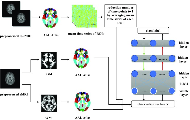
Illustration of combination of rs-fMRI, GM, and WM to discriminate ASD using DBN

Performance Measures

To evaluate the given diagnostic system, accuracy, sensitivity, specificity, and F1 score were calculated based on 10-fold cross-validation to increase the confidence level of the results. Before discussing the aforementioned criteria, it is necessary to introduce the following diagnostic conditions:

• Positive samples: children with ASD

• Negative samples: typical controls (TCs)

  • True positive (TP): the number of cases correctly labeled positive samples
  • True negative (TN): the number of cases correctly labeled negative samples
  • False positive (FP): the number of negative samples incorrectly labeled as positive
  • False negative (FN): the number of positive samples incorrectly labeled as negative

Based on the aforementioned definitions, the evaluation criteria of a classifier in medical diagnosis can be presented as follows:

• Accuracy:

$$\mathit{\text{accuracy}}=\frac{\mathit{TP}+\mathit{TN}}{\mathit{TP}+\mathit{TN}+\mathit{FP}+\mathit{FN}}$$ 9

• Sensitivity:

$$\mathit{\text{sensitivity}}=\frac{\mathit{TP}}{\mathit{TP}+\mathit{FN}}$$ 10

• Specificity:

$$\mathit{\text{specificity}}=\frac{\mathrm{T}N}{\mathit{TN}+\mathit{FP}}$$ 11

• F1 score:

$$F1\mathit{\text{score}}=\frac{2\times \mathit{TP}}{2\times \mathit{TP}+\mathit{FP}+\mathit{FN}}$$ 12

Results

In this work, subjects ranging in age from 5 to 10 years from ABIDE I and ABIDE II datasets, participated in the experiments. DBN of depths 2 (100 and 100 hidden units in the first and top layers, respectively) and 3 (100, 100, and 150 hidden units in the first, second, and the top layers, respectively) were constructed and trained. Furthermore, a diagnostic classification was done by adding a logistic regression on top of the layer of these DBN models. Pretraining and fine-tuning learning rates of 0.01 were used as hyper parameters for both DBN models. For pretraining, the stopping criteria were fixed at 50 epochs, and for fine-tuning, they were set at a maximum of 1000 epochs. In addition, the number of input dimensions of the proposed model with single data (rs-fMRI or GM or WM), integration of two data, and combination of three data are equal to 116, 232, and 348, respectively.

All the experiments were conducted using computer with an Intel Core i7 CPU (2.2 GHz) and 16 GB DDR3 memory using DBN Theano code [42]. Theano is written in Python and is also regarded as a tool for network creation using simple logic [43].

Tables 3 and 4 summarize the classification accuracies for both DBN models for unimodal and multimodal procedures. As presented in Tables 3 and 4, accuracies of 63.89% for DBN of depth 2 and 65.56% for DBN of depth 3 were obtained, when a stepwise procedure was utilized in concatenating the features of different data types. This result was obtained when the procedure was started with a single rs-fMRI modality. For DBN of depths 2 and 3, the diagnostic classification reached overall accuracies of 59.72 and 60.56% with rs-fMRI, respectively. Classification accuracy improves the most when GM (from 59.72 to 61.94% for DBN of depth 2 and 60.56 to 65% for DBN of depth 3) or WM (from 59.72 to 63.89% for DBN of depth 2 and 60.56 to 62.5% for DBN of depth 3) is added. As such, the best improvement resulted from adding WM to rs-fMRI + GM (from 65 to 65.56% for DBN of depth 3), while for DBN of depth 2, rs-fMRI + WM predicts the best accuracy among all the six data type combinations (63.89%). As a consequence, significant relationship was observed between rs-fMRI and sMRI for ASD diagnosis. For further proof of these significant relationships, in two pairwise groups (rs-fMRI + GM, rs-fMRI + WM), two-sample t test was applied on their accuracies that resulted from 10-fold cross-validation on both DBN models. According to p values, there was no significant difference between rs-fMRI and sMRI (p > 0.1 or p > 0.05) (Table 2). In this study, Python Student’s t test was used to apply the two-sample t test [44].

Table 2.

Applying t test on accuracies obtained from 10-fold cross-validation on rs-fMRI and sMRI data

Depth of DBN	p values
	fMRI-WM	fMRI-GM
2	0.7352	0.4368
3	0.8062	0.3177

Moreover, as shown in Tables 3 and 4, accuracy is improved when the depth of DBN increases from 2 to 3 in single data (rs-fMRI, GM), combination of two types of data (rs-fMRI + GM), and integration of three types of data (rs-fMRI + GM + WM). Tables 3 and 4 summarize other criteria such as sensitivity, specificity, and F1 score for both DBN models with depths 2 and 3.

Discussion

In this study, in order to classify individuals with ASD and TC for the subset of the combination of ABIDE I and ABIDE II datasets, an accuracy of 60.56% was achieved with rs-fMRI data and a maximum accuracy of 65.56% was achieved with fusion of rs-fMRI, GM, and WM data via 10-fold cross-validation on DBN of depth 3, thus achieving higher predicative performance than the shallow-architecture DBN. These findings are better than that of Nielsen et al. [15], who obtained 60.0% accuracy which was based on rs-fMRI data of ABIDE I dataset. Katuwal et al. [45], while classifying patients vs. controls using sMRI data from the ABIDE I dataset, obtained an accuracy of 60%. Ghiassian et al. [17], while classifying patients vs. controls using fMRI and sMRI data, respectively, from the ABIDE I dataset, obtained accuracies of 59.2 and 60.1%. A subset of ABIDE I participants was included in their analysis: 373 male controls and 361 male patients. It should be noted that the results of the current study are not directly comparable to the results of the study of Nielsen et al. [15], Katuwal et al. [45], and Ghiassian et al. [17], despite the fact that no results have been published on the combination of ABIDE I and ABIDE II datasets.

Based on AAL atlas, the image features used by our classifier include large regions throughout the frontal, temporal, subcortical, insula, occipital, cerebellum, and other regions (Table 5). These regions consist of a large portion of the total brain volume. The changes in GM volume are associated with ASD, particularly, in the frontal and temporal regions, the amygdala, hippocampus, caudate and other basal ganglia nuclei, and the cerebellum [46, 47]. Patients with autism were reported to exhibit reduced resting-state functional connectivity in the default mode network [48]. Many of the regions were overlapped with brain regions that were initially linked with autism. In addition, some regions are not really linked with ASD. It is possible that these regions played some unrecognized roles in autism; as a result, doing more conveying on unrecognized regions would be essential for further development of ASD diagnosis.

Table 5.

Indices and names of ROIs in the AAL template

Index	ROI label	Index	ROI label
1.2	PReCentral cyrus (PReCG)	3.4	Superior frontal gyrus (dorsal) (SFGdor)
5.6	ORBitofrontal cortex (superior) (ORBsupb)	7.8	Middle frontal gyrus (MFG)
9.10	ORBitofrontal cortex (middle) (ORBmid)	11.12	Inferier frontal gyrus (opercular) (IFGoperc)
13.14	Inferier frontal gyrus (triangular) (IFGtrang)	15.16	ORBitofrontal cortex (inferior) (ORBinf)
17.18	ROLandic operculum (ROL)	19.20	Supplementary motor area (SMA)
21.22	OLFactory (OLF)	23.24	Supperior frontal gyrus (middle) (SFGmed)
25.26	ORBitofrontal cortex (medial) (ORBmed)	27.28	RECtus gyrus (REC)
29.30	INSula (INS)	31.32	Anterior cingular gyrus (ACG)
33.34	Middle cingulate gyrus (MCG)	35.36	Posterior cingulate gyrus (PCG)
37.38	Hippocampus (HIP)	39.40	Parahippocampal gyrus (PHG)
41.42	AMYGdala (AMYG)	43.44	CALcarine cortex (CAL)
45.46	CUNeus (CUN)	47.48	LINGual gyrus (LING)
49.50	Superior occipital gyrus (SOG)	51.52	Middle occipital gyrus (MOG)
53.54	Inferior occipital gyrus (IOG)	55.56	FusiForm gyrus (FFG)
57.58	PostCentral gyrus (PoCG)	59.60	Superior parietal gyrus (SPG)
61.62	Inferior parietal lobule (IPL)	63.64	SupraMarginal gyrus (SMG)
65.66	ANGular gyrus (ANG)	67.68	PreCUNeus (PCUN)
69.70	ParaCentral lobule (PCL)	71.72	CAUdate (CAU)
73.74	PUTamen (PUT)	75.76	PALIidum (PAL)
77.78	THAlamus (THA)	79.80	HEShl gyrus (HES)
81.82	Superior temporal gyrus (STG)	83.84	Temporal POIe (superior) (TPOsup)
85.86	Middle temporal gyrus (MTG)	87.88	Temporal POIe (middle) (TPOmid)
89.90	Inferior temporal gyrus (ITG)	91–94	Crus I-II of cerebellar hemisphere (Crus)
107–108	Lobule III-X of cerebellar hemisphere (Lobule)	109–116	Lobule I-X of vermis (vermis)
Frontal = (1–16, 19–28, 69–70); insula = (29:30); temporal = (79–90); parietal = (17–18, 57–68); occipital = (43–56); Limbic = (31–40); subcortical = (41–42, 71–78); cerebellum = (91–108); vermis = (109–116)

The odd and even indices refer to the left and right hemispheric regions, respectively

DBN automatically learns complex mapping. DBN is a deep learning model that transforms the neuromorphometric features via multiple layers of nonlinear processing. At a higher abstract level, these transformations created representations that were used for the classification task. The study of Plis et al. [26] supports the notion that the depth of DBN promotes classification and increases group separation. In other words, the proposed method can successfully discover latent feature representation due to the increasing number of network layers. This is unlike the competing methods that consider only simple low-level features extracted from neuroimages. Consequently, the deep learning classifier was observed to outperform the previous methods which were used to classify individuals with ASD and TC. Moreover, in order to design a feature extractor that can transform the raw data into an appropriate feature vector, the need for careful engineering and considerable domain expertise is a major issue in conventional techniques. Deep learning gives room for a system input to be combined from raw data, thereby allowing the machine to automatically discover the representations required for machine learning tasks [49, 50]. Finally, the use of deep architectures is promoted by the application of hierarchical representations and the importance of combining unsupervised and supervised methods. In this study, due to the high dimensionality and computer resource demand required to train a DBN-based model, the raw rs-fMRI and sMRI data were not used as input data. Nevertheless, when functional and structural neuroimaging were used, the experimental results showed that the DBN-based model could achieve better differentiation performance as compared to the shallow-architecture models. Also, according to the results of the current study, there was a significant relationships between rs-fMRI, GM, and WM. In other words, the differentiation of rs-fMRI and sMRI data between individual patients and healthy controls could occur at a reasonable degree of accuracy.

With regards to a model's complexity, more computational time and resources are required by the method used in this study as compared to the previous methods. However, the computational burden of the present method is mostly involved in the computation of the training phase, which can be performed in the learning step. Otherwise, the high computational burden or complexity affects only the learning step, while the required computation for testing is a matrix vector multiplication and simple nonlinear function operations. Hence, from a clinical perspective, it is believed that there is need for more computational time and resources (only for a training phase) for higher diagnostic accuracy.

Conclusions

In conclusion, a deep learning-based feature representation was proposed based on the combined information from rs-fMRI and sMRI for ASD diagnosis. The participants of the study included subjects ranging in age from 5 to 10 years of ABIDE I and ABIDE II datasets. AAL atlas was used to parcellate rs-fMRI, GM, and WM. The best combination in terms of accuracy in the study consisted of the rs-fMRI, GM, and WM data for DBN of depth 3. As a result, there were significant relationships between rs-fMRI and sMRI. Therefore, it is recommended that MRI scanning protocols designed for the diagnosis of ASD disease be used for the collection of functional and structural MRI. In addition, this study supports an idea that increasing the depth of DBN can help improve diagnostic classification and this can perform better than shallow-architecture models. Therefore, the present study is one of the most important steps towards the development of intelligent diagnostic models. In other words, the results of this study can help doctors to identify infants or young children who are at risk of ASD before reliable behavioral symptoms manifest and plan for a better medication.

Future Direction

Based on the experience gained in this research, the following is recommended for future works and improvement of the results:

• Do research on the datasets related to a specific geographical area due to the fact that the prevalence of ASD is highly geographically dependent.

• Do research on large-scale datasets in order to achieve better results based on other criteria such as sensitivity, specificity, and F1 score.

References

- 1.Rapin I, Tuchman RF. What is new in autism? Curr Opin Neurol. 2008;21(2):143–149. doi: 10.1097/WCO.0b013e3282f49579. [DOI] [PubMed] [Google Scholar]
- 2.Mueller S, Keeser D, Reiser MF, Teipel S, Meindl T. Functional and Structural MR Imaging in Neuropsychiatric Disorders, Part 2: Application in Schizophrenia and Autism. AJNR Am J Neuroradiol. 2012;33:2033–2037. doi: 10.3174/ajnr.A2800. [DOI] [PMC free article] [PubMed] [Google Scholar]
- 3.Office of Special Education Programs, United States Department Of Education, Twenty-Seventh Annual Report to Congress on the Implementation of the Individuals with Dis- abilities Education Act, 2005.
- 4.Levy SE, Mandell DS, Schultz RT. Autism. The Lancet. 2009;374(9701):1627–1638. doi: 10.1016/S0140-6736(09)61376-3. [DOI] [PMC free article] [PubMed] [Google Scholar]
- 5.Coleman M, Gillberg C: The Autisms. Oxford; Oxford University Press, 2012
- 6.Waterhouse L. Rethinking Autism: Variation and Complexity. London: Academic Press; 2013. [Google Scholar]
- 7.Fernell E, Eriksson MA, Gillberg C. Early diagnosis of autism and impact on prognosis: a narrative review. Clin. Epidemiol. 2013;5:33–43. doi: 10.2147/CLEP.S41714. [DOI] [PMC free article] [PubMed] [Google Scholar]
- 8.Pennington Malinda L., Cullinan Douglas, Southern Louise B. Defining Autism: Variability in State Education Agency Definitions of and Evaluations for Autism Spectrum Disorders. Autism Research and Treatment. 2014;2014:1–8. doi: 10.1155/2014/327271. [DOI] [PMC free article] [PubMed] [Google Scholar]
- 9.Saniano M, Pellegrino L, Casadio M, Summa S, Garbanio E, Rossi V, Dall’Agata D, Sanguineti V, Natural interface and virtual environments for the acquisition of street crossing and path following skills in adults with Autism Spectrum Disorders: a feasibility study. J Neuroeng Rehabil, 2015. [DOI] [PMC free article] [PubMed]
- 10.Yerys BE, Pennington BF. How do we establish a biological marker for a behaviorally defined disorder? Autism as a test case. Autism Res. 2011;4(4):239–241. doi: 10.1002/aur.204. [DOI] [PubMed] [Google Scholar]
- 11.Plitt M, Barnes KA, Martin A. Functional connectivity classification of autism identifies highly predictive brain features but falls short of biomarker standards. Neuroimage Clin. 2015;7:359–366. doi: 10.1016/j.nicl.2014.12.013. [DOI] [PMC free article] [PubMed] [Google Scholar]
- 12.Mueller S, Keeser D, Reiser MF, Teipel S, Meindl T. Functional and Structural MR Imaging in Neuropsychiatric Disorders, Part 1: Imaging Techniques and Their Application in Mild Cognitive Impairment and Alzheimer Disease. AJNR Am J Neuroradiol. 2012;33:2033–2037. doi: 10.3174/ajnr.A2800. [DOI] [PMC free article] [PubMed] [Google Scholar]
- 13.Anderson JS, Nielsen JA, Froehlich AL, DuBray MB, Druzgal TJ, Cariello AN, Cooperrider JR, Zielinski BA, Ravichandran C, Fletcher PT, Alexander AL. Functional connectivity magnetic resonance imaging classification of autism. Brain. 2011;134(12):3742–3754. doi: 10.1093/brain/awr263. [DOI] [PMC free article] [PubMed] [Google Scholar]
- 14.Uddin LQ, Supekar K, Lynch CJ, Khouzam A, Phillips J, Feinstein C, Ryali S, Menon V. Salience network-based classification and prediction of symptom severity in children with autism. JAMA Psychiatry. 2013;70(8):869–879. doi: 10.1001/jamapsychiatry.2013.104. [DOI] [PMC free article] [PubMed] [Google Scholar]
- 15.Nielsen JA, Zielinski BA, et al. Multisite functional connectivity MRI classification of autism: ABIDE results. Front Hum Neurosci. 2013;7:599. doi: 10.3389/fnhum.2013.00599. [DOI] [PMC free article] [PubMed] [Google Scholar]
- 16.Chen CP, Keown CL, Jahedi A, Nair A, Pflieger ME, Bailey BA, Müller RA. Diagnostic classification of intrinsic functional connectivity highlights somatosensory, default mode, and visual regions in autism. Neuroimage Clin. 2015;8:238–245. doi: 10.1016/j.nicl.2015.04.002. [DOI] [PMC free article] [PubMed] [Google Scholar]
- 17.Ghiassian S, Greiner R, Jin P, Brown MRG. Using Functional or Structural Magnetic Resonance Images and Personal Characteristic Data to Identify ADHD and Autism. PLoS ONE. 2016;11(12):e0166934. doi: 10.1371/journal.pone.0166934. [DOI] [PMC free article] [PubMed] [Google Scholar]
- 18.Greimel E, Nehrkorn B, Schulte-Rüther M, Fink GR, Nickl-Jockschat T, Herpertz-Dahlmann B, Konrad K, Eickhoff SB. Changes in grey matter development in autism spectrum disorder. Brain Struct Funct. 2013;218(4):929–942. doi: 10.1007/s00429-012-0439-9. [DOI] [PMC free article] [PubMed] [Google Scholar]
- 19.Wilkinson M, Wang R, van der Kouwe A, Takahashi E. White and gray matter fiber pathways in autism spectrum disorder revealed by ex vivo diffusion MR tractography. Brain Behav. 2016;6(7):e00483. doi: 10.1002/brb3.483. [DOI] [PMC free article] [PubMed] [Google Scholar]
- 20.Bakhtiari R, Zürcher NR, Rogier O, Russo B, Hippolyte L, Granziera C, Araabi BN, Nili Ahmadabadi M, Hadjikhani N. Differences in white matter reflect atypical developmental trajectory in autism: A Tract-based Spatial Statistics study. Neuroimage Clin. 2012;1(1):48–56. doi: 10.1016/j.nicl.2012.09.001. [DOI] [PMC free article] [PubMed] [Google Scholar]
- 21.McCarley RW, Nakamura M, Shenton ME, Salisbury DF. Combining ERP and structural MRI information in first episode schizophrenia and bipolar disorder. Clin EEG Neurosci. 2008;39(2):57–60. doi: 10.1177/155005940803900206. [DOI] [PMC free article] [PubMed] [Google Scholar]
- 22.Michael AM, Baum SA, White T, Demirci O, Andreasen NC, Segall JM, Jung RE, Pearlson G, Clark VP, Gollub RL, Schulz SC, Roffman JL, Lim KO, Ho BC, Bockholt HJ, Calhoun VD. Does function follow form? Methods to fuse structural and functional brain images show decreased linkage in schizophrenia. Neuroimage. 2010;49(3):2626–2637. doi: 10.1016/j.neuroimage.2009.08.056. [DOI] [PMC free article] [PubMed] [Google Scholar]
- 23.Sui J, Pearlson G, Caprihan A, Adali T, Kiehl KA, Liu J, Yamamoto J, Calhoun VD. Discriminating schizophrenia and bipolar disorder by fusing fMRI and DTI in a multimodal CCA+joint ICA model. Neuroimage. 2011;57(3):839–855. doi: 10.1016/j.neuroimage.2011.05.055. [DOI] [PMC free article] [PubMed] [Google Scholar]
- 24.Sui J, He H, Yu Q, Chen J, Rogers J, Pearlson G, Mayer A, Bustillo J, Canive J, Calhoun VD, Combination of resting state fMRI, DTI, and sMRI data to discriminate schizophrenia by N-way MCCA + jICA. Fron Hum Neurosci, 7,2013. [DOI] [PMC free article] [PubMed]
- 25.Le Roux N, Bengio Y. Deep belief networks are compact universal approximators. Neural Comput. 2010;22(8):2192–2207. doi: 10.1162/neco.2010.08-09-1081. [DOI] [Google Scholar]
- 26.Plis SM, Hjelm D, Salakhutdinov R, Allen EA, Bockholt HJ, Long JD, Johnson HJ, Paulsen J, Turner JA, Calhoun VD: Deep learning for neuroimaging: a validation study. Front Neurosci, 8, 2014. [DOI] [PMC free article] [PubMed]
- 27.Suk Heung-Il, Lee Seong-Whan, Shen Dinggang. Hierarchical feature representation and multimodal fusion with deep learning for AD/MCI diagnosis. NeuroImage. 2014;101:569–582. doi: 10.1016/j.neuroimage.2014.06.077. [DOI] [PMC free article] [PubMed] [Google Scholar]
- 28.Suk HI, Lee SW, Shen D. Latent feature representation with stacked auto-encoder for AD/MCI diagnosis. Brain Struct Func. 2015;220(2):841–859. doi: 10.1007/s00429-013-0687-3. [DOI] [PMC free article] [PubMed] [Google Scholar]
- 29.Sarraf S, Tofighi G, Classification of Alzheimer’s Disease Using fMRI Data and Deep Learning Convolutional Neural Networks 2016. Available at: https://arxiv.org/pdf/1603.08631.pdf
- 30.Pang Shan, Yang Xinyi. Deep Convolutional Extreme Learning Machine and Its Application in Handwritten Digit Classification. Computational Intelligence and Neuroscience. 2016;2016:1–10. doi: 10.1155/2016/3049632. [DOI] [PMC free article] [PubMed] [Google Scholar]
- 31.Akkus Z, Galimzianova A, Hoogi A, Rubin DL, Erickson BJ. Deep Learning for Brain MRI Segmentation: State of the Art and Future Directions. J Digit Imaging. 2017;30:449–459. doi: 10.1007/s10278-017-9983-4. [DOI] [PMC free article] [PubMed] [Google Scholar]
- 32.Olshausen BA. Emergence of simple-cell receptive field properties by learning a sparse code for natural images. Nature. 1996;381:607–609. doi: 10.1038/381607a0. [DOI] [PubMed] [Google Scholar]
- 33.Hinton GE, Salakhutdinov RR. Reducing the dimensionality of data with neural networks. Science. 2006;313(5786):504–507. doi: 10.1126/science.1127647. [DOI] [PubMed] [Google Scholar]
- 34.Hinton GE, Osindero S, Teh YW. A fast learning algorithm for deep belief nets. Neural Comput. 2006;18(7):1527–1554. doi: 10.1162/neco.2006.18.7.1527. [DOI] [PubMed] [Google Scholar]
- 35.Kuang D, Guo X, An X, Zhao Y, He L: Discrimination of ADHD based on fMRI data with Deep Belief Network. In: International Conference on Intelligent Computing, Aug 3.Springer, Cham, 2014, pp 225–232
- 36.Di Martino A, Yan CG, Li Q, Denio E, Castellanos FX et al.: The autism brain imaging data exchange: towards a large-scale evaluation of the intrinsic brain architecture in autism. Mol. Psychiatry 19(6):659–667, 2014 Available at: 10.1038/mp.2013.7823774715 [DOI] [PMC free article] [PubMed]
- 37.Autism Brain Imaging Data Exchange, http://fcon_1000.projects.nitrc.org/indi/abide/, accessed at 1/10/2017
- 38.Available at: http://www.fil.ion.ucl.ac.uk/spm/software/spm8/
- 39.Jenkinson M, Smith SM: Pre-Processing of BOLD FMRI Data. Oxford University Centre for Functional MRI of the Brain (FMRIB), 2006.
- 40.Bowman F. DuBois, Guo Ying, Derado Gordana. Statistical Approaches to Functional Neuroimaging Data. Neuroimaging Clinics of North America. 2007;17(4):441–458. doi: 10.1016/j.nic.2007.09.002. [DOI] [PMC free article] [PubMed] [Google Scholar]
- 41.Tzourio-Mazoyer N, Landeau B, Papathanassiou D, Crivello F, Etard O, Delcroix N, Mazoyer B, Joliot M. Automated Anatomical Labeling of activations in SPM using a Macroscopic Anatomical Parcellation of the MNI MRI single-subject brain. NeuroImage. 2002;15(1):273–289. doi: 10.1006/nimg.2001.0978. [DOI] [PubMed] [Google Scholar]
- 42.Available at: http://deeplearning.net/tutorial/code/ (LISA lab, University of Montreal, 2015).
- 43.Erickson BJ, Korfiatis P, Akkus Z, Kline TL. Machine Learning for Medical Imaging. RadioGraphics. 2017;37(2):505–515. doi: 10.1148/rg.2017160130. [DOI] [PMC free article] [PubMed] [Google Scholar]
- 44.Available at: https://docs.scipy.org/doc/scipy-0.15.1/reference/generated/scipy.stats.ttest_ind.html
- 45.Katuwal GJ, Cahill ND, Baum SA, Michael AM: The predictive power of structural MRI in Autism diagnosis. In 37th Annual International Conference of the IEEE Engineering in Medicine and Biology Society (EMBC); 2015, p 4270–4273 [DOI] [PubMed]
- 46.Cody H, Pelphrey K, Piven J. Structural and functional magnetic resonance imaging of autism. Int J Dev Neurosci. 2002;20(3–5):421–438. doi: 10.1016/S0736-5748(02)00053-9. [DOI] [PubMed] [Google Scholar]
- 47.Bennett MR, Lagopoulos J. Neurodevelopmental sequelae associated with gray and white matter changes and their cellular basis: A comparison between Autism Spectrum Disorder, ADHD and dyslexia. Int J Dev Neurosci. 2015;46:132–143. doi: 10.1016/j.ijdevneu.2015.02.007. [DOI] [PubMed] [Google Scholar]
- 48.Minshew NJ, Keller TA. The nature of brain dysfunction in autism: functional brain imaging studies. Curr Opin Neurol. 2010;23(2):124–130. doi: 10.1097/WCO.0b013e32833782d4. [DOI] [PMC free article] [PubMed] [Google Scholar]
- 49.LeCun Y, Bengio Y, Hinton G. Deep learning. Nature. 2015;521:436–444. doi: 10.1038/nature14539. [DOI] [PubMed] [Google Scholar]
- 50.Pinaya WH, Gadelha A, Doyle OM, Noto C, Zugman A, Cordeiro Q, Jackowski AP, Bressan RA, Sato JR. Using deep belief network modelling to characterize differences in brain morphometry in schizophrenia. Sci Rep. 2016;6:38897. doi: 10.1038/srep38897. [DOI] [PMC free article] [PubMed] [Google Scholar]