

Abstract
MRI using hyperpolarized (HP) carbon-13 pyruvate is being investigated in clinical trials to provide non-invasive measurements of metabolism for cancer and cardiac imaging. In this project, we applied HP [1-13C]pyruvate dynamic MRI in prostate cancer to measure the conversion from pyruvate to lactate, which is expected to increase in aggressive cancers. The goal of this work was to develop and test analysis methods for improved quantification of this metabolic conversion. In this work, we compared specialized kinetic modeling methods to estimate the pyruvate-to-lactate conversion rate, kPL, as well as the lactate-to-pyruvate area-under-curve (AUC) ratio. The kinetic modeling included an “inputless” method requiring no assumptions regarding the input function, as well as a method incorporating bolus characteristics in the fitting. These were first evaluated with simulated data designed to match human prostate data, where we examined the expected sensitivity of metabolism quantification to variations in kPL, signal-to-noise ratio (SNR), bolus characteristics, relaxation rates, and B1 variability. They were then applied to 17 prostate cancer patient datasets.
The simulations indicated that the inputless method with fixed relaxation rates provided high expected accuracy with no sensitivity to bolus characteristics. The AUC ratio showed an undesired strong sensitivity to bolus variations. Fitting the input function as well did not improve accuracy over the inputless method. In vivo results showed qualitatively accurate kPL maps with inputless fitting. The AUC ratio was sensitive to bolus delivery variations. Fitting with the input function showed high variability in parameter maps.
Overall, we found the inputless kPL fitting method to be a simple, robust approach for quantification of metabolic conversion following HP [1-13C]pyruvate injection in human prostate cancer studies. This study also provided initial ranges of HP [1-13C]pyruvate parameters (SNR, kPL, bolus characteristics) in the human prostate.
Keywords: hyperpolarized MRI, kinetic modeling, metabolic imaging, prostate cancer, 13C-pyruvate
1 |. INTRODUCTION
MRI with hyperpolarized (HP) 13C-labeled substrates has emerged as an extremely promising metabolic imaging modality, because it can probe key metabolic pathways in patient studies.1–6 These studies utilize dissolution dynamic nuclear polarization (DNP) to enhance the 13C nuclear polarization, providing > 50 000 fold sensitivity increases in vivo.7,8 The most promising HP substrate to date is [1-13C]pyruvate, which provides the following: monitoring of a key metabolic pathway, conversion to [1-13C]lactate, which is highly upregulated in most cancer types (the “Warburg effect”); high levels of polarization via dissolution DNP; and biocompatibility at doses of 0.43 ml/kg body weight and 250mM as determined in a Phase 1 safety trial.1 Clinical translation of HP [1-13C]pyruvate was initially demonstrated in prostate cancer patients, and currently there is clinical research underway at several institutions in prostate cancer, breast cancer, brain tumors, liver metastases, and heart failure.1–5
Quantification of metabolic conversion in HP 13C MRI is a key component for the clinical application of this modality. Accurate, robust, and meaningful measurement methods are essential as HP 13C MRI enters widespread clinical trials. The robustness of the acquisition and quantification methods will be especially critical when comparing data between institutions and in multisite clinical trials. The preclinical studies performed to justify clinical studies benefited from highly reproducible experimental and physiological conditions, whereas in humans substantially more variability is a concern.
Dynamic imaging acquisition in HP 13C MRI offers the potential to provide robust quantification of metabolic conversion, regardless of differences in bolus delivery.9,10 This is in contrast to imaging at a single time-point, which can be analyzed via the lactate-to-pyruvate ratio,11 but is very dependent on experimental timing. Dynamic imaging acquisitions can be analyzed using kinetic modeling, typically to calculate a pyruvate-to-lactate metabolic conversion rate, kPL.12–23 Another popular approach is to use the area-under-curve (AUC) ratio between lactate and pyruvate that, under assumptions of constant-in-time flip angles acquired starting prior to bolus arrival or consistent bolus characteristics, is directly proportional to kPL.24
The purpose of this work was to evaluate methods for quantification of metabolism for human HP 13C MRI studies. To accomplish this, we evaluated methods in simulations that were based on the observed characteristics in human prostate cancer dynamic MR spectroscopic imaging (MRSI) studies. We also applied these methods for in vivo analysis of prostate cancer patient HP 13C-pyruvate data. The resulting kPL values are presented, along with additional experimental characteristics such as signal-to-noise ratio (SNR) and bolus parameters.
2 |. METHODS
2.1 |. Dynamic imaging
Dynamic hyperpolarized 13C MRSI was acquired for all patients analyzed in this article. They were imaged using a 3D dynamic MRSI sequence that covered the entire prostate using a blipped echo-planar spectroscopic imaging (EPSI) acquisition with a compressed sensing reconstruction,25 shown in Figure 1. This sequence used a flyback EPSI waveform with 16 encodes, a spectral resolution of 9.83-Hz and a 581-Hz spectral bandwidth. A compressed sensing reconstruction based on spectral, spatial and temporal sparsity allowed for 18-fold acceleration compared with fully sampled EPSI.
FIGURE 1.

Dynamic MRSI acquisition scheme. Data were encoded with a blipped EPSI acquisition and all time points were reconstructed together using compressed sensing.25 Excitation was performed using multiband spectral-spatial RF pulses, which applied different flip angles for pyruvate and lactate. The flip angles were also increased over time, to preserve magnetization for capturing dynamics while using all HP magnetization by the end of the experiment
Other 3D MRSI sequence parameters included 12 × 12 × 16 matrix size, TE = 6.3 ms, TR = 150 ms, 8 mm isotropic resolution, acquisition window = 42 s, and 2 s between time points. With the accelerated acquisition, only eight encodes were required per time point. Multiband spectral–spatial RF excitation pulses were used, with a lower flip angle applied to the pyruvate resonance in order to minimize saturation and maintain substrate magnetization for later time points. This results in improved SNR for the metabolic products.10 This was combined with a variable flip-angle strategy in time to use all HP magnetization.26–28 Pyruvate variable flip angles were designed with a “T1-effective” approach, using an effective decay rate of T1,eff = 35 s in Equations 6 and 7 of Xing et al28 for the flip-angle design. Lactate variable flip angles were designed using the maximum SNR formulation in Equation 8 of Nagashima,27 with an effective decay rate of 100 s for the flip-angle design. These effective decay rates for the flip-angle designs were empirically chosen to maintain the SNR for both metabolites throughout the dynamic acquisition and to provide some robustness to B1 inhomogeneity based on simulations. The flip angles used are shown in Figure 1.
The pulses were designed using minimal spectral specifications, where flip angles for [1-13C]pyruvate and [1-13C]lactate were specified by the methods described above, with all other resonances designated as “don’t-care” regions. This allowed for a relatively short duration of 4.3 ms, compared with 18–20 ms for previous designs that also had specifications for [1-13C]alanine and [1-13C]pyruvate-hydrate.10 The MATLAB software used to design these pulses is available at https://github.com/LarsonLab/Spectral-Spatial-RF-Pulse-Design.29
2.2 |. Data analysis
The primary goal of the kinetic model fitting methods was to evaluate the pyruvate-to-lactate conversion rates for our human prostate cancer imaging studies. These used the imaging methods described above. The data typically had relatively low SNR and several key experimental parameters were unknown: the in vivo metabolite relaxation rates, bolus delivery shape, and timing.
We used the tissue model shown in Figure 2, which includes an input function outside the imaging voxel and unidirectional pyruvate-to-lactate conversion via kPL within the voxel:
| (1) |
which can be described by the differential equations
| (2) |
| (3) |
FIGURE 2.

Tissue model and resulting example magnetization curves. The tissue model included an input function outside the imaging voxel, with a unidirectional input. Within the voxel, this model includes unidirectional pyruvate-to-lactate conversion via kPL and loss of magnetization due to RF pulses and relaxation. Example longitudinal and transverse magnetization curves using this model are shown, including a gamma input function, using the nominal simulation parameters of kPL = .02 /s, T1P = 30 s, T1L = 25 s, Tarrival = 4 s, Tbolus = 12 s, TR = 2 s, and the in vivo multiband variable flip-angle strategy
In this nomenclature, PZ and LZ denote the pyruvate and lactate magnetization, u is the incoming magnetization, kPL is the pyruvate-to-lactate conversion rate, and R1P = 1∕T1P, R1L = 1∕T1L are the spin-lattice relaxation rates.
To account for arbitrary flip-angle schemes, we used a hybrid discrete–continuous model.12,30 Flip-angle compensation is achieved by converting the measured signal for metabolite X at time point n, XS[n], to the Z magnetization prior to RF excitation, . The Z magnetization after RF excitation, , is also computed, and these conversions are based on the cumulative effects of the RF pulses required to acquire each image:
| (4) |
| (5) |
| (6) |
| (7) |
Nrf is the number of RF pulses used to acquire each image and θX,n[i] are the set of flip angles for metabolite X used to acquire the time-point n image.
We also assumed that the input function, u(t), was constant over each TR interval, which enabled an analytic solution to Equations 2 and 3 during the continuous period between RF pulses of our discrete–continuous model.
We compared the following metabolism quantification strategies in the framework of the above tissue model.
• Inputless kPL fitting.
This fitting approach, inspired by Khegai et al,17 only fits the lactate magnetization and not the pyruvate magnetization, where the measured pyruvate magnetization is used as the input for the kinetic model at each time point.
The estimated lactate magnetization measurement at each time point, n, is fit based only on the measured pyruvate magnetization at the adjacent time points, ,, and the estimated lactate magnetization at the previous time point by solving the two-site model in differential Equations 2 and 3:
| (8) |
where
and
This solution assumes a constant input, u[n − 1], during each time interval, TR, between time points n − 1 and n, which is computed based on the measured pyruvate magnetization:
| (9) |
The model was solved based on minimization of the least-squares error as computed between the measured and estimated lactate magnetization, , using a constrained, nonlinear least-squares solver based on a trust-region-reflective algorithm (MATLAB).
• Area-under-curve ratio24 (AUCratio).
For this method, the ratio of the area under lactate to the area under pyruvate curves is used as a simple surrogate for metabolic conversion and is computed simply as
| (10) |
Under conditions of sampling prior to arrival of the bolus and constant-in-time flip angles (i.e. not variable flip angles), this ratio is24
| (11) |
where R1L,eff is the effective lactate relaxation rate, including T1 decay, flow, conversion from lactate to pyruvate, and losses due to RF pulses.
For the multiband variable flip scheme, we computed a “calibrated AUCratio”, where predicted AUC values were computed from simulated data without noise using the nominal model parameters, including the nominal input function.
• kPL fitting with input.
In this fitting approach, the input function, u(t), was included in the fitting process and then pyruvate and lactate magnetization were fitted.
This was done using the discrete–continuous model described above to include varying flip angles. A gamma function was used for the input function, u(t):
| (12) |
with α = 4 and β = Tbolus∕4 to provide the shape shown in Figure 2.
This model had additional parameters of Tarrival, Tbolus, and ku (an input rate), which could be either fitted or fixed. The shape of the bolus can also be modified readily in this approach.
The model was solved based on minimization of the least-squares error as computed between the measured and estimated pyruvate and lactate magnetization, , using a constrained, nonlinear least-squares solver based on a trust-region-reflective algorithm (MATLAB).
• Lactate time-to-peak (TTP) and mean lactate time.
Recent work by Daniels et al14 showed that the lactate timing changes with kPL and the lactate time-to-peak (TTP) model-free approach performed indistinguishably from the best kinetic model in both their in vitro and in vivo datasets. Simulation results of the metric, as well as a ‘mean lactate time’, are described in the Supporting Information.
Constraints were placed on several parameters in the kPL fitting methods. For all results shown, these were T1L,min = 15 s, T1L,max = 35 s, Tarrival,min = 0 s, Tarrival,max = 12 s, Tbolus,min = 6 s, Tbolus,max = 10 s.
To assess the variability in arrival time between the experiments, we computed a “mean pyruvate time” as the center of mass of the pyruvate signal over time31:
| (13) |
where t[n] was the time after the nth image acquisition. This metric is reflective of the relative arrival and was chosen as it is relatively robust to noise compared with estimates of peak times which is essential given the low SNR of our data and requires no assumptions regarding the pyruvate dynamics.
Pyruvate and lactate signals were extracted from the spectra using peak area integration. The complex-valued spectra were phased separately for pyruvate and lactate, with a zero-order correction that maximized the real component across all time points. Only the real component of the integrated peak areas was used in the fitting. This phasing and peak integration provided metabolite signals with zero-mean Gaussian noise, unlike magnitude-based methods, which result in Rician noise. For Gaussian noise, least-squares minimization is equivalent to maximum-likelihood estimation.
The total SNR, tSNR, was measured for pyruvate and lactate as the summed signal divided by the standard deviation in the peak height measurements, σ, which was estimated using voxels outside the sensitive region of the RF coil that contained only noise:
| (14) |
The fitting code used in this article was implemented in MATLAB and is available in the “Hyperpolarized MRI Toolbox” at https://github.com/LarsonLab/hyperpolarized-mri-toolbox.32
2.3 |. Simulations
Simulations provide a key tool for evaluation of the proposed analysis methods, as there are no available gold-standard in vivo kPL measurements. Simulated data were generated based on a two-site model as shown above, with a gamma-distribution input function and using the same flip-angle schemes as the in vivo studies. These data were fitted as described above. Monte Carlo simulations were performed by adding Gaussian random noise to evaluate the precision and accuracy of the fitting methods. These were also performed across ranges of values for kPL, SNR, T1L, T1P, arrival time, and input function width, where the ranges were chosen based on what we observed for the human prostate cancer studies.
The nominal simulation values were kPL = .02/s, T1P = 30 s, T1L = 25 s. The simulations were normalized to have a total input magnetization of 1, and the nominal experiment had a noise standard deviation σ = 0.004. This noise level can be interpreted by noting that the theoretical maximum SNR would be 250 if all HP magnetization were captured in a single image. The gamma-distribution function was nominally set to have an arrival time 4 s after the beginning of the experiment (Tarrival = 4 s) and a full width at half-maximum of 12 s (Tbolus = 12 s), illustrated in Figure 2. The gamma-distribution function used a shape parameter α = 4 and a scaling parameter β = Tbolus∕4, which was found empirically to provide realistic bolus shapes. For AUCratio measurements, predicted AUC values were computed from simulated data without noise using the nominal model parameters, including the nominal input function.
Code for generating the simulations is available at https://github.com/agentmess/Prostate-Cancer-Analysis-Methods-Paper-2018.
2.4 |. Experiments
Imaging was performed on a GE 3T MR system on software version DV25 equipped with broad-band capabilities. For 13C, the “clamshell” transmitter consisted of a Helmholtz pair built into the patient table was used for volume excitation and was large enough to fit the entire pelvis and other coils. An endo-rectal probe containing both 13C and 1H loop coils33 was used for reception. For anatomical imaging, an additional four-channel 1H torso coil was used for reception, and the 1H body coil was used for transmit. The endo-rectal probe contained a 13C-urea (8 M, 0.6 mL) syringe in the middle of the 13C loop that was used for calibration. It was doped with gadolinium (Gd) to reduce the relaxation times to T1 = 1.0 s, T2 = 195 ms. The T1 shortening allowed for more rapid coil testing and B1 calibration prior to the pyruvate injection.
All 17 patients (63 ± 8 years old) used in this study had biopsy proven prostate cancer and received a multiparametric 1H MRI/hyperpolarized 13C MR exam prior to definitive treatment for their cancer. 12 patients, five with low grade (Gleason ≤ 3+4, serum PSA 5.2 ± 2.2 ng/ml) and seven with high grade (Gleason ≥ 4+3, serum PSA 7.1 ± 1.8 ng/ml), were enrolled in a clinical trial of hyperpolarized [1–13C]pyruvate MR prior to surgery with whole-mount step section pathology (NCT02526360). The other cohort, six patients with advanced prostate cancer (Gleason Score ≥ 4+3, serum PSA 16 ± 0.8 ng/ml), was enrolled in a clinical trial of hyperpolarized [1–13C]pyruvate MR prior to and after therapy with androgen deprivation therapy (NCT02911467).
Dissolution DNP was performed using a 5T SPINLab (GE Healthcare).7 The injected solution contained 241 ± 10mM hyperpolarized [1-13C]pyruvate polarized to 39.6 ± 4.5% and was administered at doses of 0.43 mL/kg. In the dissolution process, the 15mM electron paramagnetic agent (EPA), AH111501 (GE Healthcare), required for DNP was filtered out with mechanical filtration. An automated quality-control system evaluated pH, temperature, polarization, EPA and pyruvate concentration, and sample volume prior to injection. The resulting pH was 7.3 ± 0.4 and had an EPA concentration of 1.0 ± 0.4 μM.
In all experiments, the dynamic imaging acquisition was started 5 s after completion of the saline flush that followed the HP pyruvate injection. To improve the B0 homogeneity, we used the same shimming procedure as for our 1H MRSI clinical prostate studies.34 This begins with automatic shimming over the prostate (as selected by a PRESS selection region), followed by manual adjustments of the shim gradients to produce the peak water signal in the selection region.
For analysis, fitting was only performed in voxels with a minimum pyruvate tSNR > 80 (Equation 14). When using fixed relaxation rates in the fitting, we set T1P = 30, T1L = 25 s based on fits from the Phase I prostate cancer patient trial (T1P = 29.2 ± 5, T1L = 25.2 ± 5 s).1 Other studies in animals have measured T1P = 43 s in whole blood extracted during the experiment and T1L = 28 to 35 s in an implanted fibrosarcoma at 7T,16 and T1L ≈ 25 s with multiple fitting approaches in subcutaneous mammary adenocarcinomas at 3T.14
3 |. RESULTS
3.1 |. Simulations
3.1.1 |. Matching in vivo data
We first examined our in vivo data, and attempted to match our simulated data in order to perform relevant simulation analyses. Figure 3 shows typical data from prostate voxels, chosen to cover a representative range of kPL, SNR, and bolus characteristics, and visually matched simulated data. Examination of our in vivo data was used to choose our nominal simulation parameter values of kPL = .02/s, σ = 0.004, Tarrival = 4 s, Tbolus = 12 s, T1P = 30 s, T1L = 25 s, as well as the ranges of kPL, σ, Tarrival, and Tbolus shown in subsequent analyses.
FIGURE 3.

Examples of human prostate hyperpolarized pyruvate data from four different patient studies and corresponding simulated data with empirically matched parameters. All simulated data used T1P = 30 s and T1L = 25 s. Examples were chosen to span a range of parameters
3.1.2 |. kPL fitting with assumed bolus characteristics and relaxation rates
The simulations in Figure 4 compare the accuracy and precision of the AUCratio and kPL fitting methods using the in vivo experimental parameters and simulated across variability ranges chosen based on the in vivo fitting results (described in greater detail later). In this initial comparison, the fitting methods assumed several fixed parameters: the calibrated AUCratio was generated assuming known bolus characteristics and relaxation rates, and the fitting with input method also assumed known bolus characteristics and relaxation rates that were fixed in the fitting. The simulations with varying bolus characteristics and relaxation rates demonstrate the response to kinetic modeling with errors in these assumed parameters. The results for this are summarized in Table 1.
FIGURE 4.

Sensitivity of metabolic rate estimates based on Monte Carlo simulations for fitting methods with fixed relaxation rates and bolus characteristics. Sensitivity plots show the fractional kPL error from the kinetic models, or as predicted by an AUCratio that was calibrated for the nominal experimental parameters (pulse sequence, bolus characteristics, and relaxation rates). These are plotted over kPL, noise level, bolus arrival time (Tarrival), bolus duration (Tbolus), and metabolite relaxation rates. Accuracy/bias is shown by the solid lines, which are the average fit across the simulation. Precision/variance is shown by the dashed lines, which plot ± 1 standard deviation in the simulation fits
TABLE 1.
Summary of the simulation results shown in Figures 4, 5, and 6. The values shown are the mean average error ± the standard deviation. To highlight the weak points of each approach, values between 5 and 10% are highlighted in yellow, between 10 and 15% in orange, and > 15% in red
| Fit method | T1l | ΔkPL | ΔSNR | ΔTarrival | ΔTbolus | ΔT1L | ΔTlp | ΔB1 |
|---|---|---|---|---|---|---|---|---|
| calibrated AUCratio | Fixed | 0.4%± 10.4% | 0.2%± 4.3% | 15.6%± 3.6% | 8.3%± 3.6% | 9.5%± 3.5% | 5.5%± 3.8% | 5.6%± 3.6% |
| input-less fitting | Fixed | 1.6%± 9.3% | 1.0%± 4.7% | 0.7%± 3.7% | 0.6%± 3.8% | 10.5%± 3.6% | 0.6%± 4.0% | 10.9%± 3.9% |
| Fit | 1.4%± 15.4% | 0.9%± 10.8% | 1.2%± 10.6% | 1.1%± 10.7% | 3.1%± 9.8% | 0.9%± 10.9% | 3.7%± 7.5% | |
| fitting with input | Fixed | 0.3%± 7.0% | 0.2%± 2.9% | 11.8%± 2.5% | 8.5%± 2.4% | 8.0%± 2.4% | 8.1%± 2.5% | 1.1%± 2.4% |
| Fit | 1.6%± 10.2% | 0.5%± 5.7% | 21.6%± 3.7% | 17.0%± 4.0% | 0.8%± 4.6% | 18.5%± 4.3% | 10.4%± 3.2% | |
| Fixed | 0.2%± 8.3% | 0.2%± 4.0% | 0.2%± 3.2% | 0.2%± 3.1% | 10.0%± 3.0% | 4.4%± 3.2% | 5.9%± 3.3% | |
| Fixed | 0.6%± 8.1% | 0.3%± 3.9% | 2.9%± 2.8% | 0.8%± 2.9% | 10.1%± 3.0% | 3.9%± 3.3% | 6.4%± 3.3% | |
| Fixed | 0.3%± 8.1% | 0.1%± 3.8% | 0.3%± 3.0% | 1.2%± 3.0% | 9.5%± 2.9% | 5.5%± 3.2% | 4.1%± 3.1% | |
| Fit | 2.1%± 3.6% | 1.6%± 8.5% | 1.1%± 8.1% | 1.1%± 7.8% | 1.5%± 7.3% | 14.6%± 7.4% | 9.4%± 4.6% |
The simulations show, in the top row in Figure 4, comparable precision and accuracy between the three methods in response to variations in kPL and SNR. However, the other plots show that the methods differ in their response to variations in the bolus characteristics, relaxation rates, and B1.
The simulations show that the calibrated AUCratio is sensitive to errors in the bolus characteristics and relaxation rates for our prostate cancer experimental approach. With known bolus characteristics and relaxation rates but variation in kPL and noise (top row), the precision and accuracy of the calibrated AUCratio are comparable to those of the inputless kPL fitting. However, the AUCratio shows substantial bias with changes in all other parameters: the bolus characteristics as well as both T1P and T1L. For example, the plots show that errors in the assumed Tarrival will result in just over 20% bias in kPL at Tarrival = 0 and Tarrival = 8. Errors in the assumed bolus duration, Tbolus, lead to up to 10% bias for the range shown. Errors of ±10 s in the relaxation rates lead to approximately 10% bias in kPL. Errors in B1 of ±20% also lead to a similar 10% bias. Note that the sensitivity of the calibrated AUCratio to the bolus characteristics can be eliminated by using flip-angle schemes that are constant in time and starting before the bolus arrival, as demonstrated in the Supporting Information.
Similarly, the simulations in Figure 4 show that fitting with input that assumed known bolus characteristics and relaxation rates is also very sensitive to errors in the bolus characteristics and relaxation rates. If the bolus measurement and assumed relaxation rates are accurate, the fitting with input is accurate for the ranges of kPL and SNR shown, with a precision slightly lower than the calibrated AUCratio. However, this approach shows the largest bias when there are errors in the assumed bolus characteristics. With bolus arrival and duration errors of approximately 2 s, there is approximately 20% bias in kPL. It showed similar sensitivity to T1L errors to the other methods, but was more sensitive to T1P errors than the other methods. It was relatively insensitive to errors in B1, with < 5% bias for ±20% errors.
The inputless fitting method was the most favorable compared with the other methods in Figure 4 when fixing the bolus characteristics and relaxation rates with the chosen tissue model and experimental parameters. Unlike the other approaches, it was robust to changes in the bolus characteristics and T1P. It was also as precise as the other methods, with similar expected variances in kPL estimates. The remaining weaknesses of this method are bias, with variations in T1L and errors in the RF transmit power. Errors of ±10 s in T1L lead to 10–20% bias in kPL, while errors in B1 of ±20% also lead to a 20% bias.
3.1.3 |. kPL fitting with relaxation rate fitting
To attempt to address the bias of the fitting methods in the presence of T1L assumption errors, we also investigated inclusion of T1L fitting in Figure 5. While this does eliminate this bias for both inputless fitting and fitting with input, adding this additional fitting parameter decreases the expected precision of kPL estimates substantially. The expected standard deviation of kPL fitting is more than doubled in most situations shown. In response to ±10 s variations in T1L, the expected variance with T1L fitting is similar to the bias introduced by assuming a fixed T1L.
FIGURE 5.

Sensitivity of metabolic rate estimates for fitting methods, similar to Figure 4 (fixed bolus characteristics, fixed T1P) but with fitting T1L
3.1.4 |. kPL fitting with bolus fitting
To attempt to address the sensitivity of fitting with input to the bolus characteristics, we investigated additionally fitting the bolus characteristics instead of assuming and fixing values in Figure 6. We investigated fitting the bolus duration (Tbolus), fitting the bolus arrival time (Tarrival), and fitting both duration and arrival time.
FIGURE 6.

Sensitivity of metabolic rate estimates when using the fitting with input method, evaluating the response to fixing versus fitting the bolus parameters
These results show that all approaches reduced the sensitivity of kPL estimates to errors in the bolus characteristics. Fitting the arrival time while fixing the bolus duration, while introducing some increased bias with errors in bolus duration, provided an improvement in the expected variability. As expected, fitting the bolus duration while fixing the arrival time introduced increased bias with errors in arrival time, but provided a further improvement in the expected variability. Fitting both Tarrival and Tbolus reduced the sensitivity to Tbolus and Tarrival variations. Interestingly, fitting both parameters also had little to no penalty on the expected kPL variance across most parameters and performed comparably to fitting only one of these parameters. There was some bias when fitting both parameters, which was largest with a low SNR (σ = .01) of −5%, although it was relatively small in most cases.
3.1.5 |. kPL fitting for other flip-angle strategies
We have also applied the simulation framework for evaluating various analysis methods to other flip-angle strategies, presented in the Supporting Information. The strategies presented there include a constant 10° for all time and metabolites, as well as a “multiband” 10° (pyruvate)–20° (lactate) strategy that has been used in several prostate1 and brain5 human HP pyruvate exams.
When using fixed T1L and bolus characteristics, the inputless kPL fitting and calibrated AUCratio behave very similarly across both of the constant-in-time flip-angle strategies shown: neither suffers from bias with variations in bolus characteristics or T1P. The inputless method has improved precision slightly. Fitting with input suffers from bias with variations in bolus characteristics or T1P. All methods have bias with variations in T1L and errors in the RF transmit power.
3.2 |. Human studies
Based on the simulation results described above, we chose to apply the calibrated AUCratio, inputless kPL fitting using a fixed T1L, inputless kPL fitting including T1L fitting, and fitting with input using fixed T1L but fitting Tarrival and Tbolus to the human prostate datasets.
Sample parameter maps across a range of patients are shown in Figure 7. In general, there is a strong spatial agreement between the AUCratio and kPL from inputless fitting, both with fitting and with fixed T1L, which also showed good correspondence with T2 lesions. Mean pyruvate time maps indicate some variability in pyruvate arrival across the prostate. However, there are noticeable disagreements between the inputless kPL fitting results (labeled kPL,fixed-T1L and kPL,fit-T1L) and the fitting including bolus input characteristics, kPL,withinput. The maps for bolus arrival and duration, Tarrival and Tbolus, also showed relatively high heterogeneity, suggesting that the fitting with input was unstable in the human data.
FIGURE 7.
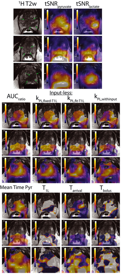
Sample in vivo maps of the metabolic AUCs as well as all fit parameters. T2 prostate lesions are highlighted by the green arrows in the T2-weighted anatomical reference images. The tSNR and kPL maps are windowed independently for each subject. The three kPL maps are windowed identically within each subject. All time values (mean time pyr, T1L, Tarrival and Tbolus) are in s and are windowed identically between subjects. Fit parameters were only computed and shown where tSNRpyruvate > 80 in order to provide reliable fits
The results of the inputless kPL fitting are summarized in Figure 8. Notably, the relationship between the calibrated AUCratio and kPL is quite variable across studies. A likely explanation for this difference is variability in pyruvate delivery time between subjects, which is expected from the simulation results in Figure 4. These showed high sensitivity of the calibrated AUCratio to variations in Tarrival and Tbolus. The mean pyruvate time values support this explanation, where studies with earlier mean pyruvate times have higher AUCratio versus kPL slope and vice versa.
FIGURE 8.

Summary of in vivo quantifications using the inputless kPL fitting with fixed T1L, where each color represents a different study. (a) Comparison of the calibrated AUCratio and kPL values from inputless fitting with a fixed T1L across all prostate voxels. Eight representative studies are shown for clear visualization. Linear fits between these parameters are shown as dashed lines. (b) Normalized histograms of the mean pyruvate time (Tμ,pyr in Equation (13)) for the same subjects as in (a), to provide a measure of pyruvate delivery time variations. (c) Comparison of the linear fitting between the calibrated AUCratio and kPL versus the average Tμ,pyr, for all 17 studies
The results of the inputless kPL fitting including T1L fitting are summarized in Figure 9. The relationship between the calibrated AUCratio and kPL was also variable across studies with this fitting approach, similarly to Figure 8. The T1L fitting in the prostate had average values within a subject between 20 and 30 s and a standard deviation of around 10 s in most subjects. This highlights the relative instability of this fitting, which is somewhat expected based on high variability in the simulation results when fitting T1L (Figure 5). Note that T1L was constrained during fitting to be between 15 and 35 s in an attempt to introduce some stability to these measurements. In the majority of voxels, the fitting hit these limits, as demonstrated by a standard deviation of around 10 s in most subjects.
FIGURE 9.

Summary of in vivo quantifications using inputless kPL fitting, with fitting T1L. (a) Comparison of the calibrated AUCratio and kPL values across all prostate voxels for the same eight representative studies as in Figure 8. Linear fits between these parameters are shown as dashed lines. (b) Mean and standard deviation of fit T1L values in the prostate from voxels with lactate tSNRlac > 20
The results of the kPL fitting with input and fixed T1L are summarized in Figure 10. The relationship between the calibrated AUCratio and kPL was also variable across studies with this fitting approach, but with more spread of kPL values compared with the inputless fitting results in Figures 8 and 9. This suggests more instability in the fitting with input. The input fit parameters Tarrival and Tbolus were correlated with each other (R2 = 0.836) and also with the mean pyruvate time metric (R2 = 0.841 between mean pyruvate time and Tarrival, R2 = 0.882 between mean pyruvate time and Tbolus). Both metrics showed notable intersubject variability in bolus delivery characteristics. There was substantial variation in Tarrival and Tbolus in the majority of subjects, suggesting relatively unstable fitting, because presumably the bolus delivery would be relatively similar within the prostate. Note that Tarrival and Tbolus were constrained during fitting to 0–12 s and 6–10 s, respectively, in an attempt to introduce some stability to these measurements.
FIGURE 10.

Summary of in vivo quantifications using kPL fitting with input and a fixed T1L. (a) Comparison of the calibrated AUCratio and kPL values across all prostate voxels for the same eight representative studies as in Figures 8 and 9. Linear fits between these parameters are shown as dashed lines. (b) Comparison of the Tbolus and Tarrival fits in the prostate across all studies, showing mean and standard deviation of both parameters. (c) Comparison of average Tbolus and Tarrival fits with the average Tμ,pyr in the prostate across all studies
Table 2 summarizes the experimental characteristics and fitting values in the prostate across all patients studied. Much like prostate cancer itself, there is a heterogeneous range of SNR, delivery, and kPL across this group.
TABLE 2.
Summary of analysis results in the prostate across all patient studies. The fit parameter values shown are based only on prostate voxel data. kPL values shown used the input-less fitting with fixed T1L
| ID | Polarization (%) | Pyr cone. (mM) | Mean pyr time (s) | Max Pyr tSNR | Max Lac tSNR | Max kPL (1/s) | mean kPL (1/s) | mean T1L (s) | mean Tarrival (s) | mean Tbolus (s) |
|---|---|---|---|---|---|---|---|---|---|---|
| 1 | 36.2 | 245 | 29.4 | 864.3 | 185.9 | 0.024 | 0.009 | 25.7 | 5.7 | 8.4 |
| 2 | 37.3 | 235 | 24.8 | 314.4 | 85.0 | 0.014 | 0.010 | 18.3 | 0.0 | 6.0 |
| 3 | 47.9 | 250 | 28.0 | 303.1 | 49.5 | 0.021 | 0.008 | 28.1 | 1.6 | 7.0 |
| 4 | 45.4 | 226 | 29.8 | 897.1 | 52.0 | 0.009 | 0.003 | 27.2 | 4.9 | 8.5 |
| 5 | 47 | 251 | 32.3 | 297.8 | 59.3 | 0.017 | 0.007 | 18.8 | 9.7 | 9.8 |
| 6 | 36.7 | 227 | 27.8 | 249.1 | 69.1 | 0.033 | 0.011 | 28.7 | 1.7 | 6.9 |
| 7 | 38.2 | 221 | 28.7 | 1415.0 | 136.4 | 0.025 | 0.009 | 25.0 | 3.5 | 8.6 |
| 8 | 40.9 | 249 | 27.5 | 1257.5 | 161.4 | 0.018 | 0.007 | 29.1 | 0.8 | 6.5 |
| 9 | 39.8 | 246 | 29.7 | 786.7 | 67.7 | 0.019 | 0.006 | 27.0 | 3.7 | 8.6 |
| 10 | 36.3 | 254 | 27.0 | 424.9 | 111.6 | 0.019 | 0.011 | 21.5 | 0.0 | 6.5 |
| 11 | 36.9 | 244 | 31.1 | 1008.5 | 66.3 | 0.021 | 0.007 | 21.8 | 7.8 | 9.5 |
| 12 | 39.1 | 241 | 30.6 | 509.5 | 61.2 | 0.024 | 0.008 | 20.1 | 4.7 | 9.2 |
| 13 | 38.1 | 225 | 29.7 | 859.4 | 120.2 | 0.014 | 0.007 | 24.4 | 3.8 | 8.4 |
| 14 | 38.5 | 246 | 29.1 | 189.2 | 141.4 | 0.049 | 0.018 | 27.4 | 3.0 | 8.1 |
| 15 | 29.8 | 251 | 29.5 | 334.0 | 62.5 | 0.023 | 0.007 | 28.7 | 5.3 | 7.7 |
| 16 | 42 | 235 | 28.0 | 703.5 | 195.5 | 0.024 | 0.011 | 27.6 | 1.1 | 6.7 |
| 17 | 43.6 | 244 | 30.0 | 276.3 | 64.4 | 0.030 | 0.008 | 26.8 | 4.5 | 8.5 |
| Mean | 39.6 | 241 | 29.0 | 628.8 | 99.4 | 0.023 | 0.009 | 25.1 | 3.6 | 7.9 |
| Std Dev | 4.5 | 10 | 1.7 | 378.1 | 48.7 | 0.009 | 0.003 | 3.6 | 2.7 | 1.1 |
4 |. DISCUSSION
In this work we evaluated approaches for quantification of metabolism in human HP [1-13C]pyruvate studies of prostate cancer patients and presented normative ranges of experimental parameters, including metabolic conversion rates. We chose to apply three methods—a calibrated AUCratio and kPL fitting with and without an input function—for quantification of pyruvate-to-lactate metabolic conversion. Part of the motivation for these methods was their simplicity, which we expected to translate into robustness for low SNR data. These were chosen from amongst numerous approaches for kinetic modeling of HP MRI data for their anticipated robustness to SNR and potential applicability to various flip-angle schemes.
The AUCratio method24 is extremely appealing in its simplicity of implementation. Under conditions of either constant-in-time flip angles acquired starting prior to bolus arrival or consistent bolus characteristics, AUCratio is proportional to kPL divided by an effective lactate relaxation rate. This proportionality breaks down when data acquisition starts after bolus arrival, and with variability in T1L that changes the effective lactate relaxation rate. To accommodate the variable flip-angle scheme, we used a calibrated AUCratio for comparisons, which was calculated based on the nominal bolus characteristics and relaxation rates. However, our results showed that this calibrated AUCratio experiences strong variability when bolus characteristics deviate from the assumed values. This was also evident from the analysis of our in vivo data, where the relationship between kPL and AUCratio was highly variable across patients. Therefore, AUCratio is not suitable for quantifying metabolism in our prostate cancer experiments.
The lactate time-to-peak (TTP) was also recently introduced as a model-free approach for estimating metabolism.14 In this prior work, lactate TTP performed indistinguishably from the best kinetic model in both in vitro and in vivo datasets. We performed simulations of this, as well as a “mean lactate time” (shown in Supporting Information), and found that both of these lactate-only model-free approaches performed poorly for the range of SNR and kPL values found in our human prostate cancer data with several flip-angle strategies. However, when we performed simulations using higher SNRs and and higher kPL values, as was the case in Daniels et al,14 the TTP and mean lactate time performed comparably to the inputless kPL fitting with fixed T1L and AUCratio, with the mean lactate time performing better than TTP with our variable flip-angle scheme. Based on these simulations, we believe these metrics are not valuable given the typical SNR and kPL values observed in our prostate cancer experiments.
Fitting of metabolic rates is often performed with either known input function or fitting of bolus characteristics, i.e. the input function parameters.13,16,20,22 We evaluated this approach in simulations, first assuming a known input function. We found that the kPL fitting was highly sensitive to errors in the assumed input function. Using this approach is also challenging for our data, as we could not consistently identify a region for estimation of an input function. It may also be more challenging to capture the bolus in our studies, due to the low pyruvate flip angles at the start of the experiments. Adding some fitting of bolus characteristics reduced the sensitivity to errors in the input function, but substantially increased the expected variance in the kPL estimates. In vivo fitting results also showed large variance in fit bolus characteristics and associated kPL maps. Therefore, we conclude that fitting including an input function was either too sensitive to errors or not precise enough to quantify metabolism in our prostate cancer experiments.
The inputless kPL fitting method, inspired by Khegai et al,17 is appealing in that it requires no explicit input function, reducing the number of parameters to fit. This fitting method only fits one or two parameters, depending on whether T1L is a free parameter. In our simulations, we found that this approach had a similar precision to both the calibrated AUCratio and kPL fitting including an input function, but with the major advantage that it was completely insensitive to the bolus characteristics. We included assumptions of fixing the relaxation rates, T1P and T1L, in this method. Simulations showed that variations in T1P do not affect the fit results. However, the remaining limitation of this approach is sensitivity to variations in T1L. While simulations indicated that fitting T1L would be an unfavorable trade-off due to the increased expected variance in kPL estimates, the in vivo results did not show any obvious increases in kPL variance. Another advantage of the inputless approach is that it can be applied readily across any acquisition strategy, i.e. for any flip angle or timing scheme. Therefore, we conclude that inputless kPL fitting was the most robust method for quantifying metabolism in our prostate cancer experiments.
We found the major limitation of the inputless kPL fitting method to be sensitivity to T1L. In the model, kPL and T1L are competing effects of the same order (0.01–0.1/s), which may make separating these poorly conditioned.35 For example, increased generation of lactate via kPL combined with an increased decay rate T1L would give somewhat similar dynamics to both rates being decreased. We chose our fixed T1L = 25 s based on modeling values from our prior prostate cancer human studies1; this was also used by Bankson et al.13 Better estimates of in vivo metabolite relaxation rates will improve the reliability of kinetic modeling. Another consideration for future work are recent studies suggesting that the intracellular T1 rates of carboxylic acids, including pyruvate and lactate, may be much shorter than those in the extracellular environment, which were reported as being as short as 10 s.36 This remains an important factor for this approach and likely many HP 13C kinetic modeling approaches, due to the poor conditioning of these models.
Another limitation of all approaches for our experimental strategy was sensitivity to flip-angle errors. The simulation results show the inputless approach is more sensitive to B1 errors compared with the fitting with input approach. One possible explanation is that the inputless fitting suffers from increased error propagation in the pyruvate signal. B1 error will introduce consistent errors in the calculation of the pyruvate state magnetization, , when it is computed directly from the actual pyruvate signal using the flip-angle compensations in Equations 4–7. The fitting with input was less sensitive to B1 errors, possibly because the pyruvate magnetization is fitted in the model and not calculated directly from the actual signal. We also suspect that some fitting methods include fit parameters that can end up compensating for B1 effects. For example, adding T1 fitting to the inputless method (Figure 5) reduces the B1 sensitivity overall. However, this is not strictly true, as when more parameters are added to the fitting with input (Figure 6), the B1 effects are worse. The bias introduced by flip-angle errors can be eliminated through B1 mapping. Fast Bloch–Siegert B1 mapping has been demonstrated for HP 13C,37–39 and more recently has been performed in real-time during the HP experiment40 to minimize bias due to inaccurate B1 calibration or unknown B1 field variations.
One potential improvement we did not explore that most certainly warrants future investigation is a tissue model that includes a vascular compartment within each imaging voxel. This has been recently investigated by Bankson et al,13 and was shown to be a more appropriate tissue model, as evaluated by the Akaike Information Criteria in preclinical study data. Similarly to this article, their work also assumed a unidirectional pyruvate-to-lactate model with fixed relaxation rates. They also used a measured vascular input function (VIF) based on pyruvate signal in the heart, as well as assumed known blood volume fractions from dynamic contrast-enhanced (DCE) MRI and pyruvate extravasation rates. This additional information likely helps to maintain model stability when including a vascular compartment within each imaging voxel, which requires assumptions or fitting of additional parameters. One reason we have not yet pursued this model is that we have not found a reliable way to estimate an input function in our prostate cancer data, but this will be the subject of future work. It may be possible to estimate the input function across all voxels in order to use a more complex tissue model.
The fitting methods and simulation evaluation framework can readily be extended to other applications beyond prostate cancer and other metabolic pathways beyond pyruvate to lactate (e.g. pyruvate to bicarbonate and/or alanine), as well as other experimental parameters. We provide guidance in the Supporting Information on modifying the simulations in the hyperpolarized-mri-toolbox.32 This framework could also be used for retrospective design of experimental parameters, such as flip angles and TR, to obtain the best estimates of kPL for expected SNR, conversion rates, relaxation rates, and bolus characteristics.
5 |. CONCLUSION
We have demonstrated the ability of MRI with hyperpolarized carbon-13 pyruvate to provide quantitative assessments of prostate cancer metabolism using dynamic imaging and kinetic modeling, and presented normative ranges of bolus delivery, SNR, and metabolic conversion rates in the prostate. This work is all based on dynamic imaging with kinetic modeling methods to provide estimates of metabolism that are independent of the bolus delivery characteristics. The AUCratio method for quantification of metabolism is robust under conditions of constant-in-time flip angles and when data are acquired starting before the bolus delivery, but is affected by variability in T1L. The inputless kPL fitting method was shown to be relatively robust for low SNR data for all flip-angle schemes and bolus characteristics, but is also sensitive to variability in T1L. There were differences of over 10 s in bolus arrival measurements across studies and several fold differences in total SNR within the prostate, and this variability must be accommodated by the acquisition and analysis methods used in future studies.
Supplementary Material
ACKNOWLEDGMENT
We thank Mary McPolin, Kimberly Okamoto, Dr Peter Shin and Dr Eugene Milshteyn for their assistance in performing the patient studies.
This work was supported by the National Institutes of Health [grant numbers R01EB017449, R01EB016741, R01CA183071, R01CA211150, and P41EB013598], as well as receiving research support from GlaxoSmithKline and GE Healthcare.
Funding information
National Institutes of Health, Grant/Award Number: R01EB017449, R01EB016741, R01CA183071, R01CA211150 and P41EB013598 © 2018 John Wiley & Sons, Ltd.
Abbreviations used:
- AUC
area-under-curve
- DCE
dynamic contrast-enhanced
- DNP
dynamic nuclear polarization
- EPSI
echo-planar spectroscopic imaging
- HP
hyperpolarized
- MRSI
MR spectroscopic imaging
- SNR
signal-to-noise ratio
- tSNR
total SNR
- TTP
time-to-peak
- VIF
vascular input function
Footnotes
SUPPORTING INFORMATION
Additional supporting information may be found online in the Supporting Information section at the end of the article.
REFERENCES
- 1.Nelson SJ, Kurhanewicz J, Vigneron DB, et al. Metabolic imaging of patients with prostate cancer using hyperpolarized [1-13C]pyruvate. Sci Transl Med 2013;5:198ra108. [DOI] [PMC free article] [PubMed] [Google Scholar]
- 2.Granlund K, Vargas HA, Lyashchenko SK, et al. Metabolic dynamics of hyperpolarized [1–13C] pyruvate in human prostate cancer In Proceedings of the World Molecular Imaging Congress. Honolulu, Hawaii; 2015: 1714–15. 10.1007/s11307-016-0968-3 [DOI] [Google Scholar]
- 3.Cunningham CH, Lau JYC, Chen AP, et al. Hyperpolarized 13C metabolic MRI of the human heart—Novelty and significance: Initial experience. Circ Res. 2016;119:1177–1182. [DOI] [PMC free article] [PubMed] [Google Scholar]
- 4.Aggarwal R, Vigneron DB, Kurhanewicz J. Hyperpolarized 1-[13C]-pyruvate magnetic resonance imaging detects an early metabolic response to androgen ablation therapy in prostate cancer. European Urol. 2017;72(6):1028–1029. [DOI] [PMC free article] [PubMed] [Google Scholar]
- 5.Park I, Larson PEZ, Gordon JW, et al. Development of methods and feasibility of using hyperpolarized carbon-13 imaging data for evaluating brain metabolism in patient studies. Magn Reson Med. 2018;80:864–873. [DOI] [PMC free article] [PubMed] [Google Scholar]
- 6.Miloushev VZ, Granlund KL, Boltyanskiy R, et al. Metabolic imaging of the human brain with hyperpolarized 13C pyruvate demonstrates 13c lactate production in brain tumor patients. Cancer Res. 2018;78(14):3755–3760. [DOI] [PMC free article] [PubMed] [Google Scholar]
- 7.Ardenkjaer-Larsen JH, Leach AM, Clarke N, Urbahn J, Anderson D, Skloss TW. Dynamic nuclear polarization polarizer for sterile use intent. NMR Biomed. 2011;24:927–932. [DOI] [PubMed] [Google Scholar]
- 8.Golman K, Zandt Ri, Lerche M, Pehrson R, Ardenkjaer-Larsen JH. Metabolic imaging by hyperpolarized 13C magnetic resonance imaging for in vivo tumor diagnosis. Cancer Res. 2006;66:10855–10860. [DOI] [PubMed] [Google Scholar]
- 9.Cunningham CH, Chen AP, Lustig M, et al. Pulse sequence for dynamic volumetric imaging of hyperpolarized metabolic products. J Magn Reson. 2008;193:139–146. [DOI] [PMC free article] [PubMed] [Google Scholar]
- 10.Larson PEZ, Kerr AB, Chen AP, et al. Multiband excitation pulses for hyperpolarized 13c dynamic chemical-shift imaging. J Magn Reson. 2008;194:121–7. [DOI] [PMC free article] [PubMed] [Google Scholar]
- 11.Albers MJ, Bok R, Chen AP, et al. Hyperpolarized 13c lactate, pyruvate, and alanine: Noninvasive biomarkers for prostate cancer detection and grading. Cancer Res. 2008;68:8607–15. [DOI] [PMC free article] [PubMed] [Google Scholar]
- 12.Bahrami N, Swisher CL, Von Morze C, Vigneron DB, Larson PEZ. Kinetic and perfusion modeling of hyperpolarized (13)C pyruvate and urea in cancer with arbitrary RF flip angles. Quant Imaging Med Surg. 2014;4:24–32. [DOI] [PMC free article] [PubMed] [Google Scholar]
- 13.Bankson JA, Walker CM, Ramirez MS, et al. Kinetic modeling and constrained reconstruction of hyperpolarized [1–13c]-pyruvate offers improved metabolic imaging of tumors. Cancer Res. 2015;75:4708–17. [DOI] [PMC free article] [PubMed] [Google Scholar]
- 14.Daniels CJ, McLean MA, Schulte RF, et al. A comparison of quantitative methods for clinical imaging with hyperpolarized 13c-pyruvate. NMR Biomed. 2016;29:387–399. [DOI] [PMC free article] [PubMed] [Google Scholar]
- 15.Harrison C, Yang C, Jindal A, et al. Comparison of kinetic models for analysis of pyruvate-to-lactate exchange by hyperpolarized 13 C NMR. NMR Biomed. 2012;25:1286–94. [DOI] [PMC free article] [PubMed] [Google Scholar]
- 16.Kazan SM, Reynolds S, Kennerley A, et al. Kinetic modeling of hyperpolarized (13)C pyruvate metabolism in tumors using a measured arterial input function. Magn Reson Med. 2013;70:943–53. [DOI] [PubMed] [Google Scholar]
- 17.Khegai O, Schulte RF, Janich MA, et al. Apparent rate constant mapping using hyperpolarized [1-(13)C]pyruvate. NMR Biomed. 2014;27:1256–65. [DOI] [PubMed] [Google Scholar]
- 18.Li LZ, Kadlececk S, Xu HN, et al. Ratiometric analysis in hyperpolarized NMR (I): Test of the two-site exchange model and the quantification of reaction rate constants. NMR Biomed. 2013;26:1308–20. [DOI] [PMC free article] [PubMed] [Google Scholar]
- 19.Mariotti E, Orton MR, Eerbeek O, et al. Modeling non-linear kinetics of hyperpolarized [1–13c] pyruvate in the crystalloid-perfused rat heart. NMR Biomed. 2016;29:377–386. [DOI] [PMC free article] [PubMed] [Google Scholar]
- 20.Sun C, Walker CM, Michel KA, Venkatesan AM, Lai SY, Bankson JA. Influence of parameter accuracy on pharmacokinetic analysis of hyperpolarized pyruvate. Magn Reson Med. 2018;79:3239–3248. [DOI] [PMC free article] [PubMed] [Google Scholar]
- 21.Witney TH, Kettunen MI, Brindle KM. Kinetic modeling of hyperpolarized 13c label exchange between pyruvate and lactate in tumor cells. J Biol Chem. 2011;286:24572–24580. [DOI] [PMC free article] [PubMed] [Google Scholar]
- 22.Zierhut ML, Yen YF, Chen AP, et al. Kinetic modeling of hyperpolarized 13c1-pyruvate metabolism in normal rats and TRAMP mice. J Magn Reson. 2010;202:85–92. [DOI] [PMC free article] [PubMed] [Google Scholar]
- 23.Xu T, Mayer D, Gu M, et al. Quantification of in vivo metabolic kinetics of hyperpolarized pyruvate in rat kidneys using dynamic 13c MRSI. NMR Biomed. 2011;24:997–1005. [DOI] [PMC free article] [PubMed] [Google Scholar]
- 24.Hill DK, Orton MR, Mariotti E, et al. Model free approach to kinetic analysis of real-time hyperpolarized 13c magnetic resonance spectroscopy data. PLoS One. 2013;e71996:8. [DOI] [PMC free article] [PubMed] [Google Scholar]
- 25.Larson PEZ, Hu S, Lustig M, et al. Fast dynamic 3D MR spectroscopic imaging with compressed sensing and multiband excitation pulses for hyperpolarized 13c studies. Magn Reson Med. 2011;65:610–9. [DOI] [PMC free article] [PubMed] [Google Scholar]
- 26.Zhao L, Mulkern R, Tseng CH, et al. Gradient-echo imaging considerations for hyperpolarized 129xe MR. J Magn Reson B. 1996;113:179–183. [PubMed] [Google Scholar]
- 27.Nagashima K Optimum pulse flip angles for multi-scan acquisition of hyperpolarized NMR and MRI. J Magn Reson. 2008;190:183–188. [DOI] [PubMed] [Google Scholar]
- 28.Xing Y, Reed GD, Pauly JM, Kerr AB, Larson PEZ. Optimal variable flip angle schemes for dynamic acquisition of exchanging hyperpolarized substrates. J Magn Reson. 2013;234:75–81. [DOI] [PMC free article] [PubMed] [Google Scholar]
- 29.Larson P, Shang H. Spectral-Spatial-RF-Pulse-Design: Version 1.2 [Electronic]. GitHub:LarsonLab, January 2018. 10.5281/zenodo.1154943. [DOI]
- 30.Maidens J, Gordon JW, Arcak M, Larson PEZ. Optimizing flip angles for metabolic rate estimation in hyperpolarized carbon-13 MRI. IEEE Trans Med Imaging. 2016;35:2403–2412. [DOI] [PMC free article] [PubMed] [Google Scholar]
- 31.Larson PEZ, Bok R, Kerr AB, et al. Investigation of tumor hyperpolarized [1–13c]-pyruvate dynamics using time-resolved multiband RF excitation echo-planar MRSI. Magn Reson Med. 2010;63:582–591. [DOI] [PMC free article] [PubMed] [Google Scholar]
- 32.Larson PEZ, Kerr AB, Milshteyn E, Zhu X, Maidens J, Gordon JW. hyperpolarized-mri-toolbox: Version 1.2; GitHub:LarsonLab, June 2018. 10.5281/zenodo.1289095 [DOI]
- 33.Tropp J, Calderon P, Vigneron DB. Systems, methods and apparatus for an endo-rectal receive-only probe. US Patent 7 945 308; 2011.
- 34.Kurhanewicz J, Vigneron D, Carroll P, Coakley F. Multiparametric magnetic resonance imaging in prostate cancer: Present and future. Curr Opin Urol. 2008;18:71–7. [DOI] [PMC free article] [PubMed] [Google Scholar]
- 35.Swisher CL, Larson PEZ, Kruttwig K, et al. Quantitative measurement of cancer metabolism using stimulated echo hyperpolarized carbon-13 MRS. Magn Reson Med. 2014;71:1–11. [DOI] [PMC free article] [PubMed] [Google Scholar]
- 36.Karlsson M, Jensen PR, Ardenkjær-Larsen JH, Lerche MH. Difference between extra- and intracellular T1 values of carboxylic acids affects the quantitative analysis of cellular kinetics by hyperpolarized NMR. Angew Chem Int Ed. 2016;55:13567–13570. [DOI] [PubMed] [Google Scholar]
- 37.Sacolick LI, Wiesinger F, Hancu I, Vogel MW. B1 mapping by Bloch–Siegert shift. Magn Reson Med. 2010;63:1315–22. [DOI] [PMC free article] [PubMed] [Google Scholar]
- 38.Schulte RF, Sacolick L, Deppe MH, et al. Transmit gain calibration for nonproton MR using the Bloch–Siegert shift. NMR Biomed. 2011;24:1068–72. [DOI] [PubMed] [Google Scholar]
- 39.Lau AZ, Chen AP, Cunningham CH. Integrated Bloch–Siegert B1 mapping and multislice imaging of hyperpolarized 13C pyruvate and bicarbonate in the heart. Magn Reson Med. 2012;67:62–71. [DOI] [PubMed] [Google Scholar]
- 40.Tang S, Milshteyn E, Gordon J, et al. A regional bolus tracking and real‐time B1 calibration method for hyperpolarized 13C MRI. Magn Reson Med. 2019;81:839–851. 10.1002/mrm.27391 [DOI] [PMC free article] [PubMed] [Google Scholar]
Associated Data
This section collects any data citations, data availability statements, or supplementary materials included in this article.