Identification of cancer driver genes based on nucleotide context

Abstract

Cancer genomes contain large numbers of somatic mutations, but few of these mutations drive tumor development. Current approaches identify driver genes based on mutational recurrence, or they approximate the functional consequences of nonsynonymous mutations using bioinformatic scores. While passenger mutations are enriched in characteristic nucleotide contexts, driver mutations occur in functional positions, which are not necessarily surrounded by a particular nucleotide context. We observed that mutations in contexts that deviate from the characteristic contexts around passenger mutations provide a signal in favor of driver genes. We therefore developed a method that combines this feature with the signals traditionally used for driver gene identification. We applied our method to whole-exome sequencing data from 11,873 tumor-normal pairs and identified 460 driver genes that clustered into 21 cancer-related pathways. Our study provides a resource of driver genes across 28 tumor types with additional driver genes identified based on mutations in unusual nucleotide contexts.

INTRODUCTION

Only a small proportion of the somatic mutations found in tumor cells drive tumor development^1-3, whereas the vast majority are functionally neutral passengers that do not confer selective advantage to cancer cells⁴. A major goal of cancer genomics is to identify these rare driver mutations amid the myriad passengers⁵. A number of highly sophisticated computational methods have been developed to identify driver mutations^6-13. Applied to thousands of tumor exomes, these methods have contributed greatly to our understanding of which genes are involved in carcinogenesis^{5,11,12,14-16}.

Current algorithms generally exploit two features of driver mutations: first they occur in functionally important genomic positions corresponding to amino acids that are critical for the protein function^6-9; and second they occur in excess over the background mutability of the genome owing to positive selection in the tumor^10-13. For most positions in the genome, functional importance is not known^17,18 and is usually proxied by differences between synonymous and nonsynonymous mutations¹², positional clustering of mutations⁷, and bioinformatically predicted scores of functional significance^8,9. To detect the excess of driver mutations over a carefully modeled background, current methods model regional variation in mutation rate with the help of synonymous mutations or epigenomic features^10-13. Recent approaches further calibrate their background models to the mutability of different nucleotide contexts^9,12,13. Typically, these methods aggregate mutation counts over genes or genomic regions, and compare them with a context-dependent background expectation^9,12,13. Current methods further combine different tests to identify driver genes, e.g. by statistical methods¹¹ or random forests¹⁹.

Nucleotide contexts around passenger mutations reflect the mutational process active in a given tumor^20-23. For instance, APOBEC enzymes scan single-stranded DNA for specific nucleotide sequence motifs and deaminate cytidine to uracil within these motifs^24-26. Similarly, mutant polymerase ε randomly introduces mutations in a non-uniform manner, since its fidelity depends strongly on the local nucleotide context^27-30. Passenger mutations are thus embedded in nucleotide contexts characteristic of the underlying mutational process^20-23, whereas driver mutations are localized towards functionally relevant positions. To the best of our knowledge, these functionally relevant positions are not surrounded by a particular nucleotide context. This suggests that driver mutations tend to occur more frequently than passengers in “unusual” nucleotide contexts, deviating from the contexts of the underlying mutational process. Consequently, an excess of mutations in unusual nucleotide contexts gauges the shift of driver mutations from functionally neutral towards functionally important positions.

Nucleotide contexts can therefore inform driver gene identification in two complementary ways. Some of the recent methods calibrated their background models to the abundance of passengers in highly mutable nucleotide contexts^9,12,13. Instead, we here examined the other end of the mutability spectrum, and assessed the sparsity of passenger mutations in “unusual” nucleotide contexts. Previous studies have focused on the enrichment of passenger mutations in process-specific nucleotide contexts^20-23, while attempts to quantify the absence of passenger mutations per nucleotide context (i.e. scoring its degree of “unusualness”) have been few. However, this is an important endeavor as it helps identify those positions in the cancer genome, in which passenger mutations are rare and mutations are thus a strong indicator of the shift of driver mutations towards functionally important positions.

The use of unusual nucleotide contexts does not require prior knowledge of the exact location of functionally relevant positions. This is essential, as the location of functionally important positions is generally unknown^17,18. We thus hypothesized that the performance of current methods to detect driver genes could be further improved by using mutations in unusual nucleotide contexts as an indirect proxy of functional importance. We developed a method that searches for genes harboring an excess of mutations in unusual nucleotide contexts, and we combined this feature with the signals used by existing methods to detect driver genes^6-13. As such, our method is well suited to identify driver genes in cancer types with both low and high background mutation rates. We demonstrate that our method expands existing catalogs of driver genes in tumors types with high background mutation rates, in which the search for drivers has proven intrinsically challenging^5,11,31,32.

RESULTS

A framework for identifying driver genes in cancer

The main steps of our method are as follows (Fig. 1a): (i) Model the mutation probability of each genomic position in the human exome depending on its surrounding nucleotide context^20-23 and the regional background mutation rate^33-35. (ii) Given a gene g with n_g nonsynonymous mutations in positions ${\overrightarrow{p}}_g$, use a Monte Carlo simulation approach^36,37 to simulate random “scenarios” in which n_g or more nonsynonymous mutations are randomly distributed along the same gene g. (iii) Compare the number and positions of mutations in each random scenario with the observed mutations in gene g. Based on these comparisons, derive a p-value for gene g (Fig. 1a). (iv) Combine this p-value with additional statistical components that test for mutational clustering and the abundance of loss-of-function mutations¹⁹, including insertions and deletions.

Fig. 1 ∣. Dependency of mutations on extended nucleotide contexts.

a, To identify driver genes, we searched for mutations in “unusual” nucleotide contexts that deviate from the context around passenger mutations. We combined this feature with other signals for driver gene identification. b, Bar graphs visualize how often each nucleotide occurs around recurrent mutations in bladder cancer (n = 317), endometrial cancer (n = 327) and melanoma (n = 582). c-d, We applied the composite likelihood model to the mutation frequency vectors of 9 COSMIC mutation signatures^11-14. For each trinucleotide context, we plotted the original frequency against the mutation frequency obtained from the composite likelihood model. e-f, We tested whether the composite likelihood model generalized to broader nucleotide contexts in 12 cancer types (bladder, n = 317; brain, n = 760; breast, n = 1443; cervix, n = 192; colorectal, n = 223; endometrial, n = 327; gastroesophageal, n = 833; head and neck, n = 425; lung adeno, n = 446; pancreas, n = 729; prostate, n = 880; skin, n = 582). For any three nucleotides in the 11-nucleotide context, we counted how many mutations were surrounded by the nucleotide triplet (n = 38,400 triplets, not necessarily adherent, ≥1 nucleotide on 5’ and 3’ sides). We plotted these counts against the prediction of the composite likelihood model. We compared original and modeled mutation frequencies by Pearson correlation coefficients (R). Plots for other mutation signatures and cancer types are provided in the supplement.

In steps (ii) and (iii), we had to evaluate the joint probability of observing n_g nonsynonymous mutations in positions ${\overrightarrow{p}}_g$ by chance, assuming they were all passengers. This probability can be expressed as a product of the probability of observing n_g nonsynonymous mutations in total, and the probability that these mutations occupy specific positions ${\overrightarrow{p}}_g$ in the gene sequence:

$$P(n_g,{\overrightarrow{p}}_g\mid s_g;{\overrightarrow{\lambda }}_g)=\underset{\text{mutation rate}}{\underset{\text{regional}}{\underbrace{P(n_g\mid s_g)}}}\cdot \underset{\text{context}}{\underset{\text{nucleotide}}{\underbrace{P({\overrightarrow{p}}_g\mid n_g;{\overrightarrow{\lambda }}_g)}}}$$ (1)

Here, P(n_g∣s_g) is the probability of observing n_g nonsynonymous mutations in gene g, given the number of synonymous mutations s_g. This factor accounts for regional variation in the background mutation rate on the megabase scale^33,34 and is based on a previous study¹³. $P({\overrightarrow{p}}_g\mid n_g;{\overrightarrow{\lambda }}_g)$ denotes the probability of these n_g nonsynonymous mutations falling in positions ${\overrightarrow{p}}_g$, conditional on their context-dependent mutability scores ${\overrightarrow{\lambda }}_g$. This factor accounts for context-specific variation in the background mutation rate on the single-base scale^20-23. We similarly computed the second factor for synonymous mutations and filtered out potential false positives caused by local deviations from the overall context-dependent distribution of passenger mutations^20,22. Finally, we determined the p-value of gene g in step (iii) as the fraction of random “scenarios” that had at least n_g nonsynonymous mutations and had a joint probability lower than that of the observed data (evaluated through equation 1).

Context-dependent mutability of genomic positions

Our method requires quantification of the mutability of genomic positions depending on their surrounding nucleotide context (${\overrightarrow{\lambda }}_g$ in the model above). To robustly characterize the mutability signal, our method first performs a Bayesian hierarchical clustering step that groups samples with similar mutational processes together (Supplementary Fig. 1). The 5’ and 3’ nucleotides immediately adjacent to a position have the strongest effect on its mutability^20-23 (Fig. 1b and Supplementary Figs. 2,3). However, as reported previously^38,39, additional upstream and downstream nucleotides flanking a position may also influence its mutability (Fig. 1b and Supplementary Figs. 2,3). Traditionally, the effect of the neighboring nucleotides has been modeled by determining the mutation probabilities of all possible 96 trinucleotide contexts independently^20-23, thus ignoring the effect of the broader nucleotide context. Here, we employed a composite likelihood model to account for the impact of flanking nucleotides outside the trinucleotide context on local mutation probabilities. In brief, this model returns a mutational likelihood score for each genomic position and integrates the effect of each flanking nucleotide as a multiplicative factor (Fig. 1c-f, Extended Data Fig. 1, Supplementary Figs. 4,5 and Supplementary Note). In particular, the composite likelihood does not model the mutability of each possible nucleotide context separately (Supplementary Figs. 6,7), which is crucial for the use of broad nucleotide contexts in the background model (sparsity of mutation counts per possible nucleotide context, prevention of overfitting of mutational hotspots in the context-dependent background signal). Applied to trinucleotide contexts, this model closely matched the mutation probabilities of the 30 widely used COSMIC mutation signatures²⁰ (Fig. 1c,d and Extended Data Fig. 1a). The composite likelihood model robustly generalized to broader nucleotide contexts for the 28 cancer types examined in this study despite signal sparsity (Fig. 1e,f, Extended Data Figs. 1-4 and Supplementary Figs. 6-11).

Considering the effects of flanking nucleotides outside of the trinucleotide context contributed to the accuracy of the composite likelihood model. Considering hepta- instead of trinucleotide contexts, for instance, increased the correlation between observed and predicted mutation probabilities of C>T mutations in melanoma from 0.76 to 0.91, thus refining the approximation of the local mutation probabilities (Extended Data Fig. 1c and Supplementary Fig. 11). Furthermore, we estimated the residual variance between predicted and observed mutability scores across nucleotide contexts as a function of the number of nucleotides included in the composite likelihood model (Extended Data Fig. 4). Accounting for extended nucleotide contexts beyond the trinucleotide context reduced the residual variance for six tumor types (bladder, breast, cervix, colorectal, endometrium, melanoma) substantially (Extended Data Fig. 4). For other tumor types, the residual variance remained largely the same when nucleotides beyond the trinucleotide context were added to the composite likelihood model. Therefore, accounting for extended nucleotide contexts in the composite likelihood model helps with the identification of nucleotide contexts at both ends of the mutability spectrum, which is important to account for the abundance of passenger mutations in “usual” nucleotide contexts, and the relative sparsity of passenger mutations in “unusual” nucleotide contexts.

Unusual contexts provide a signal for driver mutations

We next tested whether driver mutations occurred more frequently in unusual nucleotide contexts than passenger mutations, which is the biological rationale underlying our method. We first examined the nucleotide contexts around mutations in 10 known melanoma genes and 5 non-cancer-related genes (previously reported as false-positives in cancer gene discovery studies¹⁰). Most mutations in non-cancer-related genes were surrounded by the characteristic nucleotide contexts of passenger mutations, whereas several mutations in cancer genes occurred in unusual nucleotide contexts (Fig. 2a).

Fig. 2 ∣. Mutations in unusual contexts provide a signal in favor of driver genes.

a, Based on 582 melanoma samples, we examined nucleotide contexts around mutations in 10 cancer and 5 non-cancer genes. We estimated the mutability of positions using the composite likelihood. We tested which positions contained more mutations than expected (one-sided test, binomial distribution) and adjusted for multiple testing (false discovery rate, FDR). We used an FDR threshold of 0.1 to classify whether the number of mutations per position was usual (gray) or unusual (orange) compared with its surrounding nucleotide context. Each nonsynonymous mutation is visualized as a dot. A small amount of jittering was added to separate mutations in the same position. b-c, Recurrence of mutations in the same position results from passenger mutations in highly mutable contexts or driver mutations in functionally important sites. Based on 582 melanoma samples, we examined whether nucleotide contexts could distinguish between these two possibilities. We gradually modulated the mutational likelihood cutoff (x-axis) from lowly mutable to highly mutable nucleotide contexts. For each cutoff, we computed the ratio of nonsynonymous to synonymous positions (b) and the fraction of positions in established cancer genes listed in the Cancer Gene Census^42,43 (c). Error bars depict 95% confidence intervals based on the beta distribution, and dots indicate the distribution mean. As a negative control, we determined the same measures for positions without mutations. For sites with low mutational likelihood, recurrence is a better indicator of selection than for sites with high mutational likelihood.

Analogously, we next analyzed the nucleotide contexts around recurrent mutations (Fig. 2b,c). Recurrent mutations in the same position result from either driver mutations in functionally important sites^40,41, or passenger mutations accumulating in highly mutable contexts^20-23. To examine whether nucleotide contexts could help distinguish between these two possibilities, we calculated the ratio of nonsynonymous to synonymous positions (Fig. 2b), and the fraction of positions falling into established cancer genes (Fig. 2c, Cancer Gene Census^42,43). Both measures suggested that positions with recurrent mutations in lowly mutable nucleotide contexts contain higher fractions of driver mutations than positions with recurrent mutations in highly mutable contexts (Fig. 2b,c). In particular, the ratio of nonsynonymous to synonymous positions differed significantly from the baseline expectation for positions surrounded by “unusual” nucleotide contexts (P=1.47x10⁻⁴ for likelihood<0.5 based on a beta-binomial distribution). In contrast, ratios did not differ significantly from baseline for “usual” contexts (Fig. 2b, P=0.74 for likelihood<3.5). Similarly, positions with recurrent mutations in “unusual” nucleotide contexts fell into established cancer genes more frequently compared with “usual” contexts (Fig. 2c, 16.7% vs. 9.7%, P=6.48x10⁻⁴, chi-squared test). Additional analyses are presented in Supplementary Figures 12-15.

Hence, mutations in unusual nucleotide contexts provide an indirect measure of the shift of driver mutations towards functionally important positions without knowledge of their exact location. They may be particularly useful when the applicability of other proxies of functional excess is limited, owing to high abundance of functionally neutral nonsynonymous passengers (diluting the statistical power of the difference between nonsynonymous and synonymous mutations¹¹) or context-dependent positional clustering of passenger mutations (interfering with the search for driver mutations in mutational hotspots⁴⁰).

Comparison with other methods for driver gene detection

We next examined whether the rationale behind our method provided an enhanced ability to identify driver genes. For this purpose, we used whole-exome sequencing data from a collection of 11,873 tumor-normal pairs spanning 28 different tumor types (Extended Data Fig. 5 and Supplementary Table 1). Furthermore, we used two homogeneously processed datasets (TCGA and MC3, Supplementary Note) to confirm our results. We applied seven current methods for benchmarking, representing major sources for driver gene detection, including mutational recurrence above a modeled background (MutSigCV^10,11), difference between synonymous and nonsynonymous mutations (dNdScv¹²), positional clustering into mutational hotspots (OncodriveCLUST⁷), bioinformatically predicted scores of functional impact (e-Driver⁶, OncodriveFM⁸, and OncodriveFML⁹) and a combination of different sources of mutational significance (RF5 method¹⁹). We used the Cancer Gene Census (CGC)^42,43 as a conservative approximation of the true-positive rate (i.e. not every non-CGC gene is necessarily a false positive) and plotted a receiver operating characteristic (ROC) curve up to the top 1,000 significant non-CGC genes for each method.

Our method (MutPanning) exhibited the highest performance in two homogeneously processed datasets as well as our study cohort of 11,873 samples (Fig. 3, Extended Data Figs. 6-9, Supplementary Figs. 16-19). In our study cohort, our method outperformed the seven other methods in 26/28 cancer types (Extended Data Figs. 6,7 and Supplementary Fig. 16 and Supplementary Table 2), while none of the other methods displayed a robust second-best performance across all cancer types (Extended Data Fig. 6). Our method exhibited similarly improved performance relative to other methods when we used the OncoKB database⁴⁴ instead of the CGC^42,43 for comparison (Extended Data Figs. 6-8, Supplementary Fig. 17 and Supplementary Table 2). We obtained analogous results when using the precision at 5% recall⁴⁵ (Extended Data Figs. 6-8, Supplementary Fig. 18 and Supplementary Table 2) and in additional analyses (Supplementary Figs. 20-23).

Fig. 3 ∣. Comparison of different methods to identify driver genes.

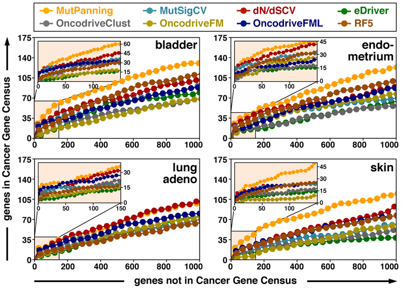
We benchmarked the performance of our method against seven other methods for driver gene identification. Since the full set of driver genes per cancer type is unknown, we used the Cancer Gene Census^42,43 (CGC) for a conservative approximation of the true-positive rate (i.e. not every non-CGC gene is necessarily a false positive). Based on the top genes returned by each method, we plotted the number of non-CGC genes (x-axis) against the number of CGC genes (y-axis) until the list contained 1,000 non-CGC genes (inset: 150 non-CGC genes). This figure shows this benchmarking analysis for three cancer types with a high context dependency based on the TCGA subcohort (bladder, n = 130; endometrium, n = 305; skin, n = 342) and one cancer type with a low context dependency based on the TCGA subcohort (lung adeno., n = 230). Similar curves for other cancer types and the full study cohort are provided in Extended Data Figures 6-9 and the supplement.

To examine whether nucleotide contexts contributed to the performance of our approach, we performed two power analyses (Supplementary Fig. 24). The impact of nucleotide contexts on the performance of MutPanning was most prominent in cancer types with highly context-specific distributions of passenger mutations (Supplementary Fig. 24). In these cancer types, extended nucleotide contexts enhanced the fit of the composite likelihood model (Extended Data Fig. 4). These analyses further suggest that mutational recurrence and unusual nucleotide contexts define complementary signals, both of which are important for the performance of MutPanning (Fig. 3, Extended Data Figs. 4, 6-9 and Supplementary Figs. 16-19, 24,25). In cancer types with low background mutation rates, such as thyroid cancer, mutational recurrence was highly informative (Fig. 3, Extended Data Figs. 4, 6-9 and Supplementary Figs. 16-19, 24,25). In cancer types with highly context-specific distributions of passenger mutations, such as melanoma, nucleotide contexts were the dominant criterion used by our method (Fig. 3, Extended Data Figs. 4, 6-9 and Supplementary Figs. 16-19, 24,25). Two cancer types (lung adenocarcinoma, squamous-cell lung cancer) with high mutation rates and context-independent distributions of passenger mutations may represent a potential challenge for MutPanning and the other methods in our benchmarking panel (Supplementary Figs. 24,25).

Stratification of driver genes based on literature support

We combined the findings identified by our method (Fig. 4-6, Extended Data Fig. 10, Supplementary Figs. 26-64 and Supplementary Tables 3,4) into a driver gene catalog of 460 genes and 827 gene-tumor pairs (pairs of significantly mutated genes and their associated tumor type). The number of gene-tumor pairs varied between tumor types (e.g., 42 pairs for cutaneous melanoma vs. 4 pairs for uveal melanoma), depending on the cohort size¹¹ (R=0.66, Fig. 4 and Supplementary Fig. 26a) and the background mutation rate⁴⁶ (R=0.24, Fig. 4 and Supplementary Fig. 26b). Furthermore, some cancer types exhibited overlaps in driver genes (Supplementary Fig. 27). Most findings could be similarly identified in the MC3^5,47 and TCGA datasets (Supplementary Fig. 28). We compared our results with both the CGC^42,43 and a systematic literature search for experimental or clinical support of our findings (Fig. 5a). Based on these comparisons, we stratified our findings into four levels based on their supporting evidence in the literature (Fig. 5a): level A includes gene-tumor pairs involving canonical cancer genes in the CGC (523/827, 63%); level B contains gene-tumor pairs with experimental literature support in the same tumor type as was identified by our method (106/827, 13%); and level C consists of gene-tumor pairs with experimental literature support in a different tumor type (level 3, 115/827, 14%). The fraction of gene-tumor pairs with no literature support (level D) varied in accordance with the false discovery rate (FDR) thresholds used for cancer gene identification: 4% for FDR<0.01, 6% for FDR<0.05, 8% for FDR<0.1, and 10% for FDR<0.25.

Fig. 4 ∣. A catalog of driver genes in human cancer.

Based on whole-exome sequencing data from 11,873 tumor-normal pairs, we derived a catalog of driver genes across 28 cancer types. Extended Data Figure 5 lists the exact number of samples per cancer type. P-values were derived by our approach (MutPanning) and then adjusted for multiple testing. The most significant gene-tumor pairs (false discovery rate < 0.25) for each cancer type are listed in decreasing order of their mutation frequencies (color of the square next to the gene name, dark red to white). A maximum of 50 gene-tumor pairs is shown per cancer type. The full catalog can be found in Supplementary Table 3. The font size of the gene name reflects its significance. We compared our driver gene catalog to four catalogs from previous pan-cancer studies. Colored dots indicate which gene-tumor pairs were listed in previous catalogs. Font colors reflect which gene-tumor pairs had been reported in the literature (confidence levels A-D). Heterogeneity in variant calling, tissue collection protocols and mutation reports (synonymous mutations were not reported for 6.1% of the samples; studies marked in Supplementary Table 1) may represent a potential limitation for driver gene identification. We therefore ran MutPanning on two uniformly processed datasets (TCGA, n = 7,060 samples, and MC3, n = 9,079 samples) that did not have these limitations. We marked gene-tumor pairs that also reached statistical significance in this smaller dataset by asterisks (*). TCGA and MC3 datasets did not include adenoid cystic carcinoma.

Fig. 6 ∣. Characterization of driver genes based on physical interactions.

a, Physical interactions between driver genes (based on 11,873 samples; identified by MutPanning) are visualized as a minimum-spanning tree based on a large-scale protein-protein interaction database⁴⁹. The color of each gene reflects its associated pathway, and the dot size indicates its maximum mutation frequency across the 28 cancer types examined in this study. b, We aggregated mutations across all driver genes in the same pathway and determined the relative contributions (dot sizes) of different pathways (rows) to the mutational landscape of 28 different cancer types (columns). The contribution of the most frequently mutated gene in each pathway is shown as a dark area within each dot.

Fig. 5 ∣. Stratification of driver genes based on literature support.

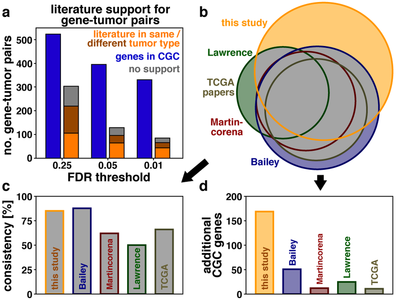
a, We stratified 827 gene-tumor pairs (based on 11,873 samples; significance values derived by MutPanning and adjusted for multiple testing) based on their literature support. Blue: gene-tumor pairs involving canonical cancer genes in the Cancer Gene Census (CGC)^34,35; orange/brown: genes-tumor pairs reported by experimental studies for the same/different tumor type as those identified by our method; gray: gene-tumor pairs with no literature support. b, Area-proportional Venn diagrams show the overlap in CGC genes between our catalog (orange) and catalogs from previous studies (green, red, blue, dark beige). The gray area reflects CGC gene-tumor pairs that were reported for the same tumor type in ≥2 independent catalogs. c, As a measure of consistency, we counted how many CGC genes from previous studies were also identified by our study (y-axis, fraction of CGC gene-tumor pairs in ≥2 independent catalogs). d, We counted the number of CGC gene-tumor pairs in our catalog that were not a part of previous studies. This measure reflects whether our catalog expanded existing catalogs by additional candidate driver genes. Our catalog (orange) recapitulated 85% of the CGC gene-tumor pairs from ≥2 previous studies (c), and contained 169 additional CGC gene-tumor pairs that were not a part of previous pan-cancer catalogs (d).

We next examined the overlap between our catalog and results reported in previous pan-cancer studies for driver gene discovery (Fig. 5b-d and Supplementary Figs. 29-32). Lawrence et al. used the MutSigCV suite to detect driver genes across 4,742 tumors¹¹. Martincorena et al. applied the dNdScv algorithm to 7,664 tumors¹². Most marker papers from The Cancer Genome Atlas (TCGA) employ MutSigCV^10,11 or MuSiC⁴⁸ to discover cancer genes^14-16. Bailey et al. recently combined 26 different computational tools to search for driver genes in 9,423 tumors⁵. We identified 85% of the CGC gene-tumor pairs reported in ≥2 of these studies. Hence, our findings are consistent with results reported previously (Fig. 5b,c). Moreover, our catalog contained 169 additional gene-tumor pairs that were part of CGC but that were missing from all previous driver gene catalogs (Figs. 4, 5b,d and Supplementary Tables 3,4). This number was larger than the corresponding numbers identified in previous studies (Lawrence¹¹: 25, Martincorena¹²: 12, TCGA^14-16: 11, Bailey⁵: 51). Both the robust performance of our method (Fig. 3, Extended Data Figs. 6-9 and Supplementary Figs. 16-19) and the marginally larger size of the sequencing dataset underlying our study (11,837 tumors in this study vs. up to 9,423 tumors in previous studies) may have contributed to the larger size of our driver gene collection. Even after removing all gene-tumor pairs identified in ≥2 studies, 47%, 50% and 84% of our findings involved canonical cancer genes in the CGC^42,43, OncoKB genes⁴⁴, or had experimental support in the literature, respectively (Fig. 5a). Analogous numbers were 40%, 42%, and 82% for genes in our catalog that were not part of any of the other driver gene catalogs. These rates are considerably higher than those obtained for random gene-tumor pairs (3.8%, 5.3%, and 17%, respectively). Moreover, several of the additional driver genes are differentially expressed between mutated and wildtype samples, a pattern that is common for known cancer genes (Supplementary Fig. 33a,b). Indeed, additional driver genes in our catalog, which were not included in any of the previous catalogs, were 5.4-fold enriched for this pattern compared with random controls (P=4.90x10⁻³⁷, chi-squared test). This adds an additional layer of support for their driver candidacy (Supplementary Fig. 33c,d). Furthermore, the protein products of the following additional genes in our catalog have known functional roles in tumor development: NOTCH2, MAML2, FGFR4, ERRFI1, FGFRL1, IKZF3, ERF, ETV6, HNF1A, CTNND2, TCF7L1, ANAPC1, BTG1, CCNQ, ROCK2, AIM2, STAT3, BIRC3, BIRC6, SF3B2, ESRP1, KLHL6, UBE2A, UBR5, POLR2A, REV3L, RECQL4, RECQL5, JMJD1C, SMARCA2, SMAD3 (cf. Supplementary Table 5 for literature references and Extended Data Fig. 10, Supplementary Figs. 34,35 and Supplementary Note for a discussion of their functional roles). Although they had been reported individually and in separate publications focusing on a certain cancer subtype or gene, they had not been identified together in a systematic pan-cancer analysis and were missing from all previous pan-cancer studies^{5,11,12,14-16}. Our full driver gene catalog is available as an online resource (www.cancer-genes.org).

Clustering of driver genes based on physical interactions

We examined whether the additional driver genes in our catalog revealed insights into tumor signaling, when analyzed in combination with established driver genes. Based on a large-scale protein-protein interaction dataset^49-52, we studied physical interactions between the protein products of established (i.e. CGC genes) and less well-established driver genes (i.e. non-CGC genes) in our catalog. We noticed that several CGC/non-CGC interactions in our catalog had well-defined functional roles in tumor signaling (Fig. 6a). For instance, the protein product of the non-CGC gene TCF7L1 directly mediates the Wnt signaling activity of CTNNB1^53,54, which is listed in the CGC; the non-CGC gene ERRFI1 encodes a protein that inhibits activation of EGFR⁵⁵ (listed in the CGC); and transcriptional activity of POLR2A (not in CGC) is mediated by MED12, which is part of the transcriptional mediator complex^56,57 and the CGC (Fig. 6a). Thus, physical interactions between protein products of CGC and non-CGC genes informed the characterization of less well-established driver genes in our catalog.

Based on their physical interactions, driver genes clustered into 21 pathways (Fig. 6a). These 21 pathways include major cancer hallmark pathways^58,59 (e.g., MAPK signaling, mTOR/PI3K signaling, cell cycle regulation, DNA repair, chromatin modification), as well as additional pathways involved in carcinogenesis (e.g., RNA binding^60,61, ribosome function^62,63, Rho GTPases^64,65, immune signaling^66,67). While some pathways were mutated across most of the 28 cancer types examined (e.g., apoptosis regulation, chromatin modification), other pathways were more specific to tumor types (e.g. G proteins, metabolism, TGFβ signaling, Wnt signaling) (Fig. 6b). Moreover, several pathways exhibited either positive (e.g. chromatin / apoptosis regulation, Wnt / TGFβ signaling, RTK / MAPK signaling) or negative (e.g. PI3K / MAPK signaling, RTK / Wnt signaling, ubiquitination / transcription factors) associations with one another (Fig. 6b). In eight pathways, >60% of the mutational signal was concentrated in ≤2 genes (e.g., mTOR/PI3K signaling, apoptosis regulation, Wnt signaling, Notch signaling). In the other 13 pathways, the signal was widely spread across rare driver genes, and <60% of the mutations occurred in the two most frequently mutated genes (e.g., chromatin modification, DNA repair, immune signaling) (Supplementary Fig. 36).

DISCUSSION

We developed a method for driver gene identification that utilizes mutations in unusual nucleotide contexts in combination with established sources for driver gene discovery (Fig. 1)^6-13. Passenger mutations are enriched in characteristic nucleotide contexts, depending on tumor type and mutational process^20-23, whereas driver mutations are localized towards functionally important positions^40,41,68,69 that do not follow any particular context-specific distribution pattern. As a result, we expect that functionally important positions occur, on average, more frequently in unusual nucleotide contexts relative to passenger mutations. Hence, a shift in mutations from “usual” to “unusual” nucleotide contexts mimics the shift from functionally neutral to functionally important positions (Figs. 1,2). Our method compares the nucleotide context around each genomic position in the human exome with the observed number of mutations at that position. Thereby, our method weighs each nonsynonymous mutation in the human exome differentially; nonsynonymous mutations in lowly mutable nucleotide contexts have a higher impact on the p-value of a gene than nonsynonymous mutations in highly mutable nucleotide contexts.

To benchmark our method, we compiled a large-scale whole-exome sequencing dataset of 11,873 samples from TCGA and non-TCGA studies (Extended Data Fig. 5). While all samples were processed with the same sequencing strategy and a homogeneous variant filter, differences in tissue collection protocols, variant calling pipelines and mutation reports (e.g., synonymous mutations were not reported in 6.1% of the samples) may represent a potential source of heterogeneity. Hence, we used two uniformly processed datasets for validation (Extended Data Fig. 9 and Supplementary Fig. 19). Furthermore, while solid tumors in TCGA were largely unaffected by tumor-in-normal contamination⁷⁰, tumor-in-normal contamination may have affected variant calling in blood tumors, thereby missing potential driver genes.

Our method enabled us to systematically aggregate large numbers of driver genes that were missing from the catalogs of previous pan-cancer studies (Figs. 4,5). For most tumor signaling pathways, mutations are spread across long tails of driver genes⁵⁸. The mutation frequencies of genes at the ends of these tails are below the detection thresholds of current methods used for driver gene identification^5,11,31,32. Since our catalog contained multiple rare driver genes with mutation frequencies as low as 1%, it may represent a valuable resource for aggregating mutations across these tails, thereby enabling driver mutations to be characterized at a pathway level rather than a gene level (Figs. 4-6). Our study further demonstrates that identifying multiple driver genes in the same pathway facilitates the biological interpretation of mutations in less well-established driver genes (Fig. 6). Our catalog may similarly inform the clinical annotation of tumor patients with mutations in less established driver genes and thereby enhance comparisons of mutation profiles across patients^51,71.

Moving forward, we anticipate that mutations in unusual nucleotide contexts may also be useful in related areas, including capturing of low-frequency mutational hotspots^40,72 and probabilistic annotation of mutations as drivers in the genomes of individual tumor patients^18,73. Furthermore, our approach may directly inform driver gene identification in ongoing and future large-scale cancer genome sequencing efforts, such as GENIE⁷⁴, MSK-IMPACT⁷⁵, PCAWG⁷⁶, ICGC⁷⁷, and HMF⁷⁸. Our method is available as an interactive software tool called MutPanning (www.cancer-genes.org) and can be run online as a module on the GenePattern platform^79,80 (www.genepattern.org).

ONLINE METHODS

Sequencing data curation and variant filtering

We compiled whole-exome sequencing data from 32 TCGA-related projects (7,091 samples), as well as from 55 TCGA-independent publications (4,856 samples). Mutation annotation files (MAF) for TCGA-related projects were directly obtained from the TCGA Gene Data Analysis Center (GDAC) data portal hosted by the Broad Institute (gdac.broadinstitute.org, latest data version from 01/28/2016, doi:10.7908/C11G0KM9). MAF files for TCGA-independent studies were either downloaded from the cBioPortal platform (cbioportal.org^81,82) or - if not available there - directly from the supplement of the publications. Details on how we selected these studies and samples can be found in the Supplementary Note.

We integrated all mutations into a combined MAF file and removed duplicate patients from the combined MAF file. We grouped patients into subcohorts according to their cancer type. Most of these tumor types were defined as in the TCGA marker papers (27/28 tumor types).

Finally, mutations from this combined MAF file were processed through a homogeneous filtering step, in order to minimize sequencing artifacts, mutation calling errors, and germline variants that might have slipped through the variant filters applied in each study. We applied the following filters:

Filtering of common germline variants:

Each mutation was compared against the Exome Aggregation Consotrium (ExAC) database⁸³, which reports germline variants of 60,706 individuals. As similarly described previously,⁷⁴ we removed all variants from the MAF file that occurred more than 10 times in any of the 7 ExAC subpopulations.

Removal of OxoG and strand bias sequencing artifacts:

The 8-oxoguanine (OxoG) artifact results from excessive oxidation during sequence library preparation⁸⁴, whereas the strand bias artifact produces disparities between G>T and C>A mutation counts at low variant allele frequencies⁴⁷. We used the annotation of the MC3 dataset⁴⁷ in order to reduce OxoG and strand bias artifacts from our MAF file.

Removal of low quality samples:

Samples for which >10% of the somatic mutations were flagged as artifacts or germline variants were entirely removed from the study.

In this way, we arrived at a study cohort of 11,873 tumor samples, spanning 28 different cancer types.

Statistical analyses to identify driver genes

The first step of MutPanning is to cluster samples with similar passenger mutation distributions together and to characterize the context-dependent background signal in each cluster. In brief, we first counted the number of mutations of each base substitution type t (C>A, C>G, C>T, T>A, T>C, T>G) for each sample and summarized these counts into a type count vector $v^{\text{type}}\in {\mathbb{N}}^6$. Each element $v_t^{\text{type}}$ in this vector corresponds to the number of base substitutions of type t ∈ {1, …, 6}. To capture the extended nucleotide context around mutations, we further counted the nucleotides that occurred in a 20-nucleotide window around the mutations identified for each sample. We summarized these counts into the nucleotide context count vector $v^{\text{seq}}\in {\mathbb{N}}^{6\times 20\times 4}$. Each element $v_{t,p,n}^{\text{seq}}$ in this vector denotes the count of nucleotide n ∈ {A, C, G, T} in position p ∈ [−10; 10]]{0} around mutations of type t ∈ {1, …, 6}. MutPanning then quantified the similarity between two count vectors v, $w\in {\mathbb{N}}^l$ by examining whether updating a distribution prior x by w made the observation of v more likely (Dirichlet-multinomial distribution). More details on the choice of the distribution prior x as well as the metrics to compare count vectors are provided in the Supplementary Note.

In the second step MutPanning establishes a composite likelihood model for each cluster $\mathcal{C}$ of samples. In brief, MutPanning derives likelihood ratios for each cluster $\mathcal{C}$ as

$${\lambda }_{t,p,n}^{\mathcal{C}}≔\frac{v_{t,p,n}^{\text{seq}}}{v_t^{\text{type}}\cdot f_{n(t),p,n}^{\text{ref}}}$$

$v_t^{\text{type}}$ denotes the number of mutations of type t ∈ {1, …, 6} in cluster $\mathcal{C}$. $v_{t,p,n}^{\text{seq}}$ denotes the number of mutations type t ∈ {1, …, 6}, that are surrounded by nucleotide n ∈ {A, C, G, T} in position p ∈ [−10; 10]\{0}. Further, $f_{n,p,n^{\prime }}^{\text{ref}}$ denotes the frequency of nucleotide n′ around nucleotide n at position p in the human exome. n(t) denotes the reference nucleotide of base substitution type t (i.e. C for types t = 1,2,3 and T for types t = 4,5,6). Hence, ${\lambda }_{t,p,n}^{\mathcal{C}}$ reflects the ratio of the observed number of mutations ($v_{t,p,n}^{\text{seq}}$) and the number of mutations ($v_t^{\text{type}}\cdot f_{n(t),p,n}^{\text{ref}}$), if all mutations were equally distributed across the human exome.

Similarly, given a substitution type t ∈ {1, …, 6} we define the likelihood ratio as

$${\lambda }_t^{\mathcal{C}}≔\frac{v_t^{\text{type}}}{\mid v^{\text{type}}\mid ∕6}$$

with ∣v∣ := Σ_k∣v_k∣. Hence, ${\lambda }_t^{\mathcal{C}}$ reflects the ratio of the observed number of mutations ($v_t^{\text{type}}$) of substitution type t and the number of mutations (∣v^type∣/6), if all substitution types occurred at the same frequency.

Given a base substitution type t and a genomic position that is surrounded by nucleotides n_p at position p, we define its composite likelihood as

$${\lambda }_{\text{pos}}≔{\lambda }_t^{\mathcal{C}}\cdot \prod _{\underset{p\ne 0}{-10\le p\le 10}}{\lambda }_{t,p,n_p}^{\mathcal{C}}$$

for reference nucleotides n₀ = C, T and

$${\lambda }_{\text{pos}}≔{\lambda }_t^{\mathcal{C}}\cdot \prod _{\underset{p\ne 0}{-10\le p\le 10}}{\lambda }_{t,\text{-}p,\overline{n_p}}^{\mathcal{C}}$$

for reference nucleotides $n_0=\mathrm{A},\mathrm{G}.\overline{n_p}$ denotes the complementary nucleotide to n_p.

This likelihood score indicates whether the position is expected to contain more (λ_pos > 1) or fewer mutations (λ_pos < 1) compared with a flat mutation distribution. That way, highly mutable nucleotide contexts (λ_pos ≫ 1) and mutations in highly unusual nucleotide contexts (λ_pos ≪ 1) can be identified and weighted differently in the statistical model. More details on the full composite likelihood model can be found in the Supplementary Note.

In the third step MutPanning examines, for each gene, how likely the number and positions of its nonsynonymous mutations might occur by chance. For each reference nucleotide, three different base substitutions are possible. Hence, given a gene of length l_g, we defined a count vector $v^g\in {\mathbb{N}}^{l_g\times 3}$ that contains the number of mutations at each position and for each substitution type. Similarly, we defined the vector λ^g that contains the composite likelihood for each position and substitution type in gene g. We then split these vectors into v^g = (v^g,s, v^g,n) and λ^g = (λ^g,s, λ^g,n), reflecting synonymous and nonsynonymous positions, respectively.

MutPanning then determines the probability of observing v^g,n by chance, given the number of synonymous mutations ∣v^g,s∣ and the context-dependent composite likelihood scores λ^g,n in the same gene. This probability factorizes into two factors

$$P(\mid v^{g,\mathrm{n}}\mid \mid \mid v^{g,\mathrm{s}}\mid )\cdot P(v^{g,\mathrm{n}}\mid \mid v^{g,\mathrm{n}}\mid ;{\lambda }^{g,\mathrm{n}})$$

The first factor ($P(\mid v^{g,\mathrm{n}}\mid \mid \mid v^{g,\mathrm{s}}\mid )$) reflects the chance of observing ∣v^g,n∣ nonsynonymous mutations in a gene with ∣v^g,s∣ synonymous mutations. This factor is modeled by a convoluted Poisson distribution, i.e. ∣v^g,n∣ ~ Pois(μ), where the mutation rate μ is drawn from another distribution, conditional on the number of synonymous mutations ∣v^g,s∣ (cf. Supplementary Note for more details). This factor accounts for mutational recurrence above the regional background mutation rate. The second factor ($P(v^{g,\mathrm{n}}\mid \mid v^{g,\mathrm{n}}\mid ;{\lambda }^{g,\mathrm{n}})$) reflects the chance that these ∣v^g,n∣ nonsynonymous mutations occur in their observed positions (v^g,n) conditional on the context-dependent mutational likelihood scores λ^g,n. This factor is modeled by a Multinomial distribution that distributes the ∣v^g,n∣ nonsynonymous mutations across genomic positions proportionally to their composite likelihood scores in λ^g,n. This factor accounts for excess of mutations in unusual nucleotide contexts. This enabled us to obtain the probability of observing the number (first factor) and positions (second factor) of nonsynonymous mutations by chance. More details on these distribution models are provided in the Supplementary Note.

In the fourth step MutPanning examines whether the probability derived in the previous step is small or large compared with a “random” scenario of ≥ ∣v^g,n∣ nonsynonymous mutations in the same gene obtained from Monte Carlo simulations. For each scenario, we randomly drew the total number of nonsynonymous mutations from a randomized Poisson model¹³, conditional on the number of synonymous mutations ∣v^g,s∣. We simulated the positions of nonsynonymous mutations across the gene based on a multinomial distribution, conditional on the context-dependent composite likelihood scores λ^g,n (cf. Supplementary Note for more details on both distributions). To derive a p-value for each gene, we compared the probability of each scenario with the observed number and positions of nonsynonymous mutations (cf. Supplementary Note for more details on this comparison). More details on the simulation step and the computation of p-values are provided in the Supplementary Note.

In the fifth step MutPanning computes two additional p-values for each gene that account for destructive mutations (which are an important source to detect tumor suppressors) and for positional clustering (which is an important source to detect mutational hotspots in oncogenes). These p-values are then combined with the p-value from the previous step using the Brown method. More details on the calculation of these additional p-values and their combination to a final p-value are provided in the Supplementary Note.

In the last step MutPanning adjusts its significance values for multiple testing (false-discovery rate). Furthermore, it performs additional filtering steps to reduce the number of false positives. For instance, MutPanning determines whether nucleotide contexts around synonymous mutations deviate from the overall distribution pattern (e.g. due to local accumulation of APOBEC-related mutations). If the null hypothesis is locally violated (local deviation from the context-dependent distribution), significant p-values do not necessarily reflect positive selection and these genes are filtered. More details on this filtering step as well as the adjustment for multiple testing can be found in the Supplementary Note.

Stratification of driver genes based on literature support

To explore the relevance of our findings, we systematically examined which significantly mutated genes were supported by the literature. In brief, we stratified our findings by four different “confidence” levels:

Level A: The gene was listed as a canonical cancer gene in the Cancer Gene Census (CGC)^42,43.

Level B: The gene had not previously been reported as significantly mutated, but there was experimental data implicating the gene in the tumor type in which we discovered it as significantly mutated.

Level C: The gene had not been previously reported, and there was no experimental data to support the gene in the tumor type in which we discovered it. However, there was experimental data that the gene has a functional role in cancer.

Level D: The gene had not been previously reported as significantly mutated, and there was no experimental evidence that this gene plays a role in cancer.

To characterize the functional roles of significant findings that were not part of the CGC^42,43 (level A), we systematically searched for publications with experimental and clinical data that casually implicated our findings in cancer. In brief, our literature search proceeded in two main stages. The first stage entailed searching for experimental evidence in the same tumor type in which we had detected the gene as significantly mutated (Steps 1a-4a). In the second stage, we examined whether genes for which we had not found any functional data in the same tumor type, had been reported as functionally relevant in any cancer type (Steps 1b-4b).

Both of these stages contained a fully automated part (steps 1-3) and a manual review part (step 4). In steps 1-3 we automatically retrieved abstracts of publications supporting our findings from the PubMed database, pre-filtered them, and sorted them by relevance. In step 4 we determined whether the publications contained any experimental data to support our findings.

Step 1a: For each gene-tumor pair, we searched for the gene name plus the cancer type through the Esearch tool (NCBI Entrez Programming Utilities, E-utilities). The Esearch tool provided automated access to the Pubmed database. For the gene name, we used the officially approved symbol from the NCBI Reference Sequence Database (RefSeq). For the name of the cancer type, we used all names that commonly appear in the literature (Supplementary Note). If more than one name existed, we searched for all names separately and combined the search results. That way, we obtained for each gene-tumor pair a list of PubMed IDs (PMIDs). If we retrieved more than 100 IDs, we added the search term “mutation” to narrow our results.

Step 1b: We proceeded in parallel to step 1a. Instead of the cancer type, we used the search terms “cancer”, “tumor”, “tumour”, and “carcinoma”.

Steps 2a/b: For each PMID from steps 1a and 1b, we obtained the abstracts and meta-information from the PubMed database through the Efetch tool (NCBI E-utilities). Based on this information, we pre-filtered our results to guarantee that an abstract in English was available and that the PMID referred to original work. Reviews and case reports were excluded if annotated in the meta-data.

Step 3a/b: For several gene-tumor pairs, we obtained more abstracts than we could manually review. Hence, we retained a maximum of 15 publications per gene-tumor pair for manual review. To retain the most relevant publications, we prioritized abstracts according to the relevance score (Supplementary Information). We further sorted publications with the same relevance score by the number of citations, which we retrieved through the Elink tool (NCBI E-utilities; link name: “pubmed_ pubmed_citedin”). As a third criterion, we used the publication date.

Steps 4 a/b: We manually reviewed the abstracts to examine whether the publication reported experimental data for the gene-tumor pair. In particular, we excluded publications that only co-mentioned the tumor type and the gene name in the abstract or reported the presence of a somatic mutation without any functional validation. In addition, we excluded all publications that reported germline mutations, e.g., associated the gene with increased cancer risk or heritability. As a negative control, we ran the entire literature search pipeline for 2,500 randomly chosen gene-tumor pairs, i.e., randomly chosen combinations of arbitrary genes in the RefSeq database and an arbitrary cancer type examined in this study.

More details on these steps as well as a visualization of our search strategy can be found in the Supplementary Note.

Analysis of mutations in unusual nucleotide contexts

In Figure 2 we visualized the “unusualness” of nucleotide contexts for mutations in 10 known melanoma genes and 5 non-cancer genes. To quantify whether a position contained more mutations than expected based on its surrounding nucleotide context, we counted the number v_i of mutations in each position i, compared these counts with the mutational likelihood λ_i in position i. To this end, we determined for each position with v_i mutations the probability of observing v_i or more mutations in position i by chance, based on a binomial distribution

$$p_i≔\sum _{v_i\le k\le v}\left(\begin{array}{c}\hfill v\hfill \\ \hfill k\hfill \end{array}\right)\cdot {\left(\frac{{\lambda }_i}{\lambda }\right)}^k\cdot {\left(1-\frac{{\lambda }_i}{\lambda }\right)}^{v-k}$$

where v Σv_i and λ = Σλ_i denote the sum of counts and mutational likelihoods across all positions in the gene.

We then adjusted these probabilities p_i for multiple testing. We randomly distributed v mutations across the gene based on a multinomial distribution with probabilities λ_i/λ. For each position, we determined a p-value with the same equation as above. We repeated this procedure 100 times to generate a cumulative distribution function of the expected distribution of p-values. For each observed p-value p_i, we determined the expected p-value ${\tilde{p}}_i$ at the same rank based on the distribution of simulated p-values. We then determined the fraction f_i of simulated p-values that were smaller than p_i. Similarly, we computed the fraction ${\tilde{f}}_i$ of simulated p-values that were smaller than ${\tilde{p}}_i$. We then derived the ratio $f_i∕{\tilde{f}}_i$ and defined the q-value of p_i as the minimum of that ratio and all following q-values. For each nonsynonymous mutation, we then plotted the q-value of its position against its genomic coordinate in the gene, where we used an FDR cutoff of 0.1 to classify a mutation as usual (q ≥ 0.1) vs. unusual (q < 0.1).

Analysis of physical interactions between driver genes

For Figure 6 we used experimental data from the STRING database⁴⁹ to study physical interactions between driver genes in our catalog. The STRING database collects experimental interaction data from BIND⁸⁵, DIP⁸⁶, GRID⁸⁷, HPRD⁸⁸, IntAct⁸⁹, MINT⁹⁰, and PID⁹¹ datasets, and assigns to each interaction a unified score between 0 (no interaction) and 1 (strong interaction). We asked whether physical interactions with established driver genes might inform the characterization of less well-established driver genes.

We visualized physical interactions between driver genes in our catalog as a minimum spanning tree based on Kruskal’s algorithm. In brief, Kruskal’s algorithm starts with a separate unconnected component for each gene. The algorithm then goes through all physical interactions in descending order. If a physical interaction connects two unconnected components, it is added as an edge to the graph, otherwise it is ignored. This procedure is analogous to hierarchical clustering with single-linkage. We then used force-directed graph drawing (Fruchterman-Reingold algorithm) to align nodes and physical interactions between them.

Visualization of mutations using protein crystal structures

Protein structures were visualized using The PyMOL Molecular Graphics System, Version 2.0 Schrödinger, LLC and the respective publicly available coordinate files derived from The Protein Data Bank (PDB). In detail, X-ray diffraction crystal structures of CEBPA (PDB: 1NWQ⁹²), GATA3 (PDB: 4HCA⁹³), RUNX1 (PDB: 1H9D⁹⁴), and SOX17 (PDB: 4A3N superposed with 3F27^95,96), as well as electron microscopy structures of ANAPC1 (PDB: 5G05⁹⁷), and POLR2A (5IYB⁹⁸) were utilized. All protein sequences were Homo sapiens except for CEBPA, which was Rattus norvegicus (sequence homology to H. sapiens CEBPA: 93.1%). The crystalized human sequence of SOX17 was superimposed with the crystal structure of Mus musculus SOX17 in complex with DNA. No structural differences between human (no DNA) and mouse SOX17 (plus DNA) were observed. HDAC4 is a co-crystalized structure with a selective Class IIa HDAC inhibitor (not shown) occupying the active site of the deacetylase.

Extended Data

Extended Data Fig. 1. Modeling of mutation probabilities based on extended nucleotide contexts.

a, We applied the composite likelihood model to COSMIC mutation signatures. For each trinucleotide context, we compared the original mutation frequency against the mutation frequency returned by the composite likelihood model based on Pearson correlation. Dot colors reflect base substitution types. b, For six base substitution types, we plotted the original mutation probability (based on 11873 samples) against the prediction of the composite likelihood model, which we derived as the product of the mutational likelihood of its reference nucleotide and its substitution type. Each dot represents a cancer type. Pearson correlations are annotated at the bottom right. The number of samples per cancer type can be found in Extended Data Figure 5. c, For three cancer types (bladder, n = 317 samples; endometrium, n = 327; skin, n = 582) we examined whether nucleotides outside the trinucleotide context affected mutation probabilities. For this purpose, we compared mutation probabilities, modeled based on tri- (blue) and 7-nucleotide contexts (yellow), with original mutation probabilities based on context-specific mutation counts. Data points are sorted according to the modeled mutation rates, derived from the 7-nucleotide context (x-axis). Black circles indicate ratios between the observed probabilities and the corresponding trinucleotide-specific likelihoods (y-axis). Similarly, the orange line displays the ratio between the likelihoods, derived from the 7-nucleotide and trinucleotide contexts, respectively (y-axis). Local mutation probabilities vary across positions surrounded the same trinucleotide context. Accounting for extended nucleotide contexts reduces this heterogeneity.

Extended Data Fig. 2. Evaluation of the composite likelihood model applied to extended nucleotide contexts.

To test the independence assumption of the composite likelihood model, we examined the interaction between any two positions (25 possible combinations) in the 11-nucleotide context around mutations of eight cancer types (bladder, n = 317 samples; breast, n = 1443; colorectal, n = 223; endometrium, n = 327; gastroesophageal, n = 833; head and neck, n = 425; lung adeno, n = 446; skin, n = 582). For any two positions, there are 96 possible nucleotide contexts and we plotted the observed mutation count of each nucleotide context (x-axis) against the predictions of the composite likelihood model (y-axis). Pearson correlation coefficients between observed and predicted data served as a measure of interaction. Each position pair is visualized in a separate correlation plot, and positions are annotated at the bottom right of the plot. For instance, pair (−1,1) refers to the trinucleotide context. Dot colors indicate the base substitution types.

Extended Data Fig. 3. Generalization of the composite likelihood model to extended nucleotide contexts.

We counted the number of mutations in each possible nucleotide context of length ≤7 based on the sequencing data of 11,873 samples. The exact number of samples per cancer type included in this analysis is shown in Extended Data Figure 5. We compared these counts with the mutability scores returned by the composite likelihood model (218,448 different nucleotide contexts). Since the number of possible nucleotide contexts was too large to be visualized directly, we plotted the data point density. The Pearson correlation coefficient (R) of each plot is annotated at the bottom right.

Extended Data Fig. 4. Extended nucleotide contexts contribute to the performance of the composite likelihood model.

We examined whether accounting for extended contexts beyond trinucleotide contexts improved the fit of the composite likelihood model. To this end, we varied the number of nucleotides in the composite likelihood model between 0 (i.e. only substitution types) and 6 (i.e. 7-nucleotide contexts). We computed the residual sum of squared differences between observed mutation counts and the predictions of the composite likelihood model. As a negative control, we determined the residual sum of squares for a uniform distribution. This baseline was used to normalize the residual sum of squares for each cancer type. For some cancer types with “flat” mutation signatures, nucleotide contexts only had minor impact on the fit of the model, but did not decrease the performance of the model (e.g., lung adeno., n = 446 samples). For other cancer types, the fit of the model largely depended on the trinucleotide context, but not on the extended nucleotide context (e.g., prostate cancer, n = 880). For most cancer types with high background mutation rates, the fit of the composite likelihood model strongly depended on the extended nucleotide context (e.g., bladder, n = 317; breast, n = 1443; cervical, n = 192; colorectal, n = 223; endometrial cancer, n = 327; melanoma, n = 582).

Extended Data Fig. 5. A large-scale cohort of whole-exome sequencing data to identify rare cancer genes.

To systematically identify candidate cancer genes, we analyzed sequencing data from 11,873 individual tumor samples using the statistical framework that we had developed in this study. Our study cohort contained whole-exome sequencing data from 32 TCGA-related (orange) and 55 TCGA-independent (blue) projects.

Extended Data Fig. 6. Benchmarking of the performance of MutPanning for cancer gene identification.

We benchmarked the performance of our method against 7 previously published methods for cancer gene identification based on the sequencing data of 11,873 samples spanning 28 different cancer types. The exact number of samples per cancer type can be found in Extended Data Figure 5. To benchmark the performance of a method, we sorted genes according to the significance values (adjusted for multiple testing) returned by the method. As a conservative approximation of the true-positive rate we used Cancer Gene Census (CGC) genes (a, b, c) and OncoKB genes (d, e, f) to derive ROC and precision-recall curves. We quantified the performance of each method as the area under the ROC curve (AUC) for the top 150 (a, d) or 1000 (b, e) non-CGC/OncoKB genes, respectively. Further, we determined the precision at 5% recall for each method (c, f). We normalized these measures to the maximum within each cancer type.

Extended Data Fig. 7. Comparison of different methods for cancer gene identification.

We benchmarked the performance of our method against 7 previously published methods for cancer gene identification based on the sequencing data of 11,873 samples spanning 28 different cancer types. To benchmark the performance of a method, we sorted genes according to the significance values (adjusted for multiple testing) returned by the method. As a conservative approximation of the true-positive rate we used Cancer Gene Census (CGC) genes (a, c, e) and OncoKB genes (b, d, f) to derive ROC and precision-recall curves. We quantified the performance of each method as the area under the ROC curve (AUC) for the top 150 (a, b) or 1000 (c, d) non-CGC/OncoKB genes, respectively. Further, we determined the precision at 5% recall for each method (e, f). Box plots indicate the distribution of these performance measures for each method across cancer types. Each cancer type is represented by a dot. Boxes indicate the 25%/75% interquartile range, whiskers extend to the 5%/95%-quantile range. The median of each distribution is indicated as a vertical line.

Extended Data Fig. 8. Comparison of performance measures derived from CGC vs. OncoKB.

We benchmarked the performance of our method against 7 previously published methods for cancer gene identification based on the sequencing data of 11,873 samples spanning 28 different cancer types. To benchmark the performance of a method, we sorted genes according to the significance values (adjusted for multiple testing) returned by the method. As a conservative approximation of the true-positive rate we used Cancer Gene Census (CGC) genes and OncoKB genes to derive ROC and precision-recall curves. We quantified the performance of each method as the area under the ROC curve (AUC) for the top 150 (a) or 1000 (b) non-CGC/OncoKB genes, respectively. Further, we determined the precision at 5% recall for each method (c). This figure compares the performance measures derived from the CGC (x-axis) and OncoKB (y-axis) databases. Each dot represents the AUC/precision of a different method (dot color) for an individual cancer type. The concordance between CGC and OncoKB measures suggests that our measure of performance does not entirely depend on the dataset used to approximate the true-positive rate.

Extended Data Fig. 9. Comparison of methods in two homogeneously processed datasets.

We compared the performance of MutPanning with 7 other methods on two independently processed datasets (TCGA subcohort (a-c, g-i), n = 7060 samples; MC3 dataset (d-f, j-l), n = 9079). We used the Cancer Gene Census (CGC) (a-f) and OncoKB (g-l) for benchmarking. We quantified the performance by the AUC of the ROC curve of the top 1,000 non-CGC/OncoKB genes returned by each method. a, d, g, j, Box plots indicate the distribution of performance measures for each method. Boxes indicate the 25%/75% interquartile range, whiskers extend to the 5%/95%-quantile range. Distribution medians are indicated as vertical lines. Each dot represents an AUC for one of the 27 cancer types in the TCGA and MC3 datasets. b, e, h, k, We normalized AUCs by the maximum AUC within each tumor type. We then compared these normalized AUCs between methods across cancer types. c, f, i, l, We compared the AUCs obtained from our original study cohort with the AUCs from TCGA and MC3 based on Pearson correlation. Each dot reflects a cancer type/method. Cohort sizes for TCGA/MC3 datasets: bladder: 130/386; blood: 197/139; brain: 576/821; breast: 975/779; cervix: 192/274; cholangio: 35/34; colorectal: 223/316; endometrium: 305/451; gastroesophageal: 467/529; head&neck: 279/502; kidney clear: 417/368; kidney non-clear: 227/340; liver: 194/354; lung adenocarcinoma: 230/431; lung squamous: 173/464; lymph: 48/37; ovarian: 316/408; pancreas: 149/155; pheochromocytoma: 179/179; pleura: 82/81; prostate: 323/477; sarcoma: 247/204; skin: 342/422; testicular: 149/145; thymus: 123/121; thyroid: 402/492; uveal melanoma: 80/80

Extended Data Fig. 10. Recurrent mutations in domains of protein-DNA interaction.

Significance values in this figure legend were computed using MutPanning and adjusted for multiple testing (false discovery rate, FDR). Recurrent SOX17 mutations in endometrial cancer (n = 327 samples, FDR = 8.77x10⁻³) are located in the high-mobility-group box domain at the SOX17-DNA interface (PDB: 4A3N superposed with 3F27). POLR2A harbors recurrent mutations in lung adenocarcinoma (n = 446, FDR = 9.28x10⁻⁶) at the end of an alpha helical segment that is directly pointed at the major groove of the double stranded DNA (PDB: 5IYB). The open complex of a cryo-EM multicomponent structure where the melted single-stranded template DNA is inserted into the active site and RNA polymerase II locates the transcription start site is visualized. CEBPA harbors recurrent mutations in hematological malignancies (n = 1018, FDR = 1.16x10⁻⁷) at the cross-over interface of the two CEBPA homodimers (PDB: 1NWQ). GATA3 (PDB: 4HCA) harbors recurrent mutations in breast cancer (n = 1443, FDR < 10⁻²⁰) at Asn334, which is located in the GATA-type 2 zinc finger (res317-res341), as well as the residue Met294, which is located peripheral to the GATA-type 1 zinc finger domain (res263-res287). RUNX1 harbors recurrent mutations in breast cancer (n = 1443, FDR = 2.22x10⁻⁴) and hematological malignancies (n = 1018, FDR = 1.94x10⁻⁵). Arg174 plays an important role for DNA recognition and facilitates the formation of hydrogen bond interactions to a guanosine base from the consensus DNA binding sequence of RUNX1 (PDB: 1H9D).

References

- 1.Stratton MR, Campbell PJ & Futreal PA The cancer genome. Nature 458, 719–24 (2009). [DOI] [PMC free article] [PubMed] [Google Scholar]
- 2.Vogelstein B et al. Cancer genome landscapes. Science 339, 1546–58 (2013). [DOI] [PMC free article] [PubMed] [Google Scholar]
- 3.Stephens PJ et al. The landscape of cancer genes and mutational processes in breast cancer. Nature 486, 400–4 (2012). [DOI] [PMC free article] [PubMed] [Google Scholar]
- 4.Greaves M & Maley CC Clonal evolution in cancer. Nature 481, 306–13 (2012). [DOI] [PMC free article] [PubMed] [Google Scholar]
- 5.Bailey MH et al. Comprehensive Characterization of Cancer Driver Genes and Mutations. Cell 173, 371–385 e18 (2018). [DOI] [PMC free article] [PubMed] [Google Scholar]
- 6.Porta-Pardo E & Godzik A e-Driver: a novel method to identify protein regions driving cancer. Bioinformatics 30, 3109–14 (2014). [DOI] [PMC free article] [PubMed] [Google Scholar]
- 7.Tamborero D, Gonzalez-Perez A & Lopez-Bigas N OncodriveCLUST: exploiting the positional clustering of somatic mutations to identify cancer genes. Bioinformatics 29, 2238–44 (2013). [DOI] [PubMed] [Google Scholar]
- 8.Gonzalez-Perez A & Lopez-Bigas N Functional impact bias reveals cancer drivers. Nucleic Acids Res 40, e169 (2012). [DOI] [PMC free article] [PubMed] [Google Scholar]
- 9.Mularoni L, Sabarinathan R, Deu-Pons J, Gonzalez-Perez A & Lopez-Bigas N OncodriveFML: a general framework to identify coding and non-coding regions with cancer driver mutations. Genome Biol 17, 128 (2016). [DOI] [PMC free article] [PubMed] [Google Scholar]
- 10.Lawrence MS et al. Mutational heterogeneity in cancer and the search for new cancer-associated genes. Nature 499, 214–218 (2013). [DOI] [PMC free article] [PubMed] [Google Scholar]
- 11.Lawrence MS et al. Discovery and saturation analysis of cancer genes across 21 tumour types. Nature 505, 495–501 (2014). [DOI] [PMC free article] [PubMed] [Google Scholar]
- 12.Martincorena I et al. Universal Patterns of Selection in Cancer and Somatic Tissues. Cell 171, 1029–1041 e21 (2017). [DOI] [PMC free article] [PubMed] [Google Scholar]
- 13.Weghorn D & Sunyaev S Bayesian inference of negative and positive selection in human cancers. Nat Genet 49, 1785–1788 (2017). [DOI] [PubMed] [Google Scholar]
- 14.Hoadley KA et al. Multiplatform analysis of 12 cancer types reveals molecular classification within and across tissues of origin. Cell 158, 929–944 (2014). [DOI] [PMC free article] [PubMed] [Google Scholar]
- 15.Cancer Genome Atlas Research, N. Comprehensive molecular profiling of lung adenocarcinoma. Nature 511, 543–50 (2014). [DOI] [PMC free article] [PubMed] [Google Scholar]
- 16.Hoadley KA et al. Cell-of-Origin Patterns Dominate the Molecular Classification of 10,000 Tumors from 33 Types of Cancer. Cell 173, 291–304 e6 (2018). [DOI] [PMC free article] [PubMed] [Google Scholar]
- 17.Cooper GM & Shendure J Needles in stacks of needles: finding disease-causal variants in a wealth of genomic data. Nat Rev Genet 12, 628–40 (2011). [DOI] [PubMed] [Google Scholar]
- 18.Kircher M et al. A general framework for estimating the relative pathogenicity of human genetic variants. Nat Genet 46, 310–5 (2014). [DOI] [PMC free article] [PubMed] [Google Scholar]
- 19.Kumar RD, Searleman AC, Swamidass SJ, Griffith OL & Bose R Statistically identifying tumor suppressors and oncogenes from pan-cancer genome-sequencing data. Bioinformatics 31, 3561–8 (2015). [DOI] [PMC free article] [PubMed] [Google Scholar]
- 20.Alexandrov LB et al. Signatures of mutational processes in human cancer. Nature 500, 415–21 (2013). [DOI] [PMC free article] [PubMed] [Google Scholar]
- 21.Alexandrov LB et al. Mutational signatures associated with tobacco smoking in human cancer. Science 354, 618–622 (2016). [DOI] [PMC free article] [PubMed] [Google Scholar]
- 22.Nik-Zainal S et al. Mutational processes molding the genomes of 21 breast cancers. Cell 149, 979–93 (2012). [DOI] [PMC free article] [PubMed] [Google Scholar]
- 23.Nik-Zainal S et al. Landscape of somatic mutations in 560 breast cancer whole-genome sequences. Nature 534, 47–54 (2016). [DOI] [PMC free article] [PubMed] [Google Scholar]
- 24.Ebrahimi D, Alinejad-Rokny H & Davenport MP Insights into the motif preference of APOBEC3 enzymes. PLoS One 9, e87679 (2014). [DOI] [PMC free article] [PubMed] [Google Scholar]
- 25.Roberts SA et al. Clustered mutations in yeast and in human cancers can arise from damaged long single-strand DNA regions. Mol Cell 46, 424–35 (2012). [DOI] [PMC free article] [PubMed] [Google Scholar]
- 26.Roberts SA et al. An APOBEC cytidine deaminase mutagenesis pattern is widespread in human cancers. Nat Genet 45, 970–6 (2013). [DOI] [PMC free article] [PubMed] [Google Scholar]
- 27.Church DN et al. DNA polymerase epsilon and delta exonuclease domain mutations in endometrial cancer. Hum Mol Genet 22, 2820–8 (2013). [DOI] [PMC free article] [PubMed] [Google Scholar]
- 28.Shinbrot E et al. Exonuclease mutations in DNA polymerase epsilon reveal replication strand specific mutation patterns and human origins of replication. Genome Res 24, 1740–50 (2014). [DOI] [PMC free article] [PubMed] [Google Scholar]
- 29.Goodman MF & Fygenson KD DNA polymerase fidelity: from genetics toward a biochemical understanding. Genetics 148, 1475–82 (1998). [DOI] [PMC free article] [PubMed] [Google Scholar]
- 30.Ganai RA & Johansson E DNA Replication-A Matter of Fidelity. Mol Cell 62, 745–55 (2016). [DOI] [PubMed] [Google Scholar]
- 31.Hofree M et al. Challenges in identifying cancer genes by analysis of exome sequencing data. Nat Commun 7, 12096 (2016). [DOI] [PMC free article] [PubMed] [Google Scholar]
- 32.Tokheim CJ, Papadopoulos N, Kinzler KW, Vogelstein B & Karchin R Evaluating the evaluation of cancer driver genes. Proc Natl Acad Sci U S A 113, 14330–14335 (2016). [DOI] [PMC free article] [PubMed] [Google Scholar]
- 33.Makova KD & Hardison RC The effects of chromatin organization on variation in mutation rates in the genome. Nat Rev Genet 16, 213–23 (2015). [DOI] [PMC free article] [PubMed] [Google Scholar]
- 34.Schuster-Bockler B & Lehner B Chromatin organization is a major influence on regional mutation rates in human cancer cells. Nature 488, 504–7 (2012). [DOI] [PubMed] [Google Scholar]
- 35.Polak P et al. Reduced local mutation density in regulatory DNA of cancer genomes is linked to DNA repair. Nat Biotechnol 32, 71–5 (2014). [DOI] [PMC free article] [PubMed] [Google Scholar]
- 36.North BV, Curtis D & Sham PC A note on the calculation of empirical P values from Monte Carlo procedures. Am J Hum Genet 71, 439–41 (2002). [DOI] [PMC free article] [PubMed] [Google Scholar]
- 37.Ewens WJ On estimating P values by the Monte Carlo method. Am J Hum Genet 72, 496–8 (2003). [DOI] [PMC free article] [PubMed] [Google Scholar]
- 38.Shiraishi Y, Tremmel G, Miyano S & Stephens M A Simple Model-Based Approach to Inferring and Visualizing Cancer Mutation Signatures. PLoS Genet 11, e1005657 (2015). [DOI] [PMC free article] [PubMed] [Google Scholar]
- 39.Fredriksson NJ et al. Recurrent promoter mutations in melanoma are defined by an extended context-specific mutational signature. PLoS Genet 13, e1006773 (2017). [DOI] [PMC free article] [PubMed] [Google Scholar]
- 40.Chang MT et al. Identifying recurrent mutations in cancer reveals widespread lineage diversity and mutational specificity. Nat Biotechnol 34, 155–63 (2016). [DOI] [PMC free article] [PubMed] [Google Scholar]
- 41.Chang MT et al. Accelerating Discovery of Functional Mutant Alleles in Cancer. Cancer Discov 8, 174–183 (2018). [DOI] [PMC free article] [PubMed] [Google Scholar]
- 42.Forbes SA et al. COSMIC: exploring the world's knowledge of somatic mutations in human cancer. Nucleic Acids Res 43, D805–11 (2015). [DOI] [PMC free article] [PubMed] [Google Scholar]
- 43.Futreal PA et al. A census of human cancer genes. Nat Rev Cancer 4, 177–83 (2004). [DOI] [PMC free article] [PubMed] [Google Scholar]
- 44.Chakravarty D et al. OncoKB: A Precision Oncology Knowledge Base. JCO Precis Oncol 2017(2017). [DOI] [PMC free article] [PubMed] [Google Scholar]
- 45.Grau J, Grosse I & Keilwagen J PRROC: computing and visualizing precision-recall and receiver operating characteristic curves in R. Bioinformatics 31, 2595–7 (2015). [DOI] [PMC free article] [PubMed] [Google Scholar]
- 46.Tomasetti C, Marchionni L, Nowak MA, Parmigiani G & Vogelstein B Only three driver gene mutations are required for the development of lung and colorectal cancers. Proc Natl Acad Sci U S A 112, 118–23 (2015). [DOI] [PMC free article] [PubMed] [Google Scholar]
- 47.Ellrott K et al. Scalable Open Science Approach for Mutation Calling of Tumor Exomes Using Multiple Genomic Pipelines. Cell Syst 6, 271–281 e7 (2018). [DOI] [PMC free article] [PubMed] [Google Scholar]
- 48.Dees ND et al. MuSiC: identifying mutational significance in cancer genomes. Genome Res 22, 1589–98 (2012). [DOI] [PMC free article] [PubMed] [Google Scholar]
- 49.Szklarczyk D et al. STRING v10: protein-protein interaction networks, integrated over the tree of life. Nucleic Acids Res 43, D447–52 (2015). [DOI] [PMC free article] [PubMed] [Google Scholar]
- 50.Cowen L, Ideker T, Raphael BJ & Sharan R Network propagation: a universal amplifier of genetic associations. Nat Rev Genet 18, 551–562 (2017). [DOI] [PubMed] [Google Scholar]
- 51.Hofree M, Shen JP, Carter H, Gross A & Ideker T Network-based stratification of tumor mutations. Nat Methods 10, 1108–15 (2013). [DOI] [PMC free article] [PubMed] [Google Scholar]
- 52.Leiserson MD et al. Pan-cancer network analysis identifies combinations of rare somatic mutations across pathways and protein complexes. Nat Genet 47, 106–14 (2015). [DOI] [PMC free article] [PubMed] [Google Scholar]
- 53.Murphy M, Chatterjee SS, Jain S, Katari M & DasGupta R TCF7L1 Modulates Colorectal Cancer Growth by Inhibiting Expression of the Tumor-Suppressor Gene EPHB3. Sci Rep 6, 28299 (2016). [DOI] [PMC free article] [PubMed] [Google Scholar]
- 54.Morrison G, Scognamiglio R, Trumpp A & Smith A Convergence of cMyc and beta-catenin on Tcf7l1 enables endoderm specification. EMBO J 35, 356–68 (2016). [DOI] [PMC free article] [PubMed] [Google Scholar]
- 55.Cairns J et al. Differential roles of ERRFI1 in EGFR and AKT pathway regulation affect cancer proliferation. EMBO Rep 19(2018). [DOI] [PMC free article] [PubMed] [Google Scholar]
- 56.Taatjes DJ The human Mediator complex: a versatile, genome-wide regulator of transcription. Trends Biochem Sci 35, 315–22 (2010). [DOI] [PMC free article] [PubMed] [Google Scholar]
- 57.Soutourina J Transcription regulation by the Mediator complex. Nat Rev Mol Cell Biol 19, 262–274 (2018). [DOI] [PubMed] [Google Scholar]
- 58.Garraway LA & Lander ES Lessons from the cancer genome. Cell 153, 17–37 (2013). [DOI] [PubMed] [Google Scholar]
- 59.Hanahan D & Weinberg RA Hallmarks of cancer: the next generation. Cell 144, 646–74 (2011). [DOI] [PubMed] [Google Scholar]
- 60.Pereira B, Billaud M & Almeida R RNA-Binding Proteins in Cancer: Old Players and New Actors. Trends Cancer 3, 506–528 (2017). [DOI] [PubMed] [Google Scholar]
- 61.Neelamraju Y, Gonzalez-Perez A, Bhat-Nakshatri P, Nakshatri H & Janga SC Mutational landscape of RNA-binding proteins in human cancers. RNA Biol 15, 115–129 (2018). [DOI] [PMC free article] [PubMed] [Google Scholar]
- 62.Pelletier J, Thomas G & Volarevic S Ribosome biogenesis in cancer: new players and therapeutic avenues. Nat Rev Cancer 18, 51–63 (2018). [DOI] [PubMed] [Google Scholar]
- 63.Sulima SO, Hofman IJF, De Keersmaecker K & Dinman JD How Ribosomes Translate Cancer. Cancer Discov 7, 1069–1087 (2017). [DOI] [PMC free article] [PubMed] [Google Scholar]
- 64.Wilson KF, Erickson JW, Antonyak MA & Cerione RA Rho GTPases and their roles in cancer metabolism. Trends Mol Med 19, 74–82 (2013). [DOI] [PMC free article] [PubMed] [Google Scholar]
- 65.Porter AP, Papaioannou A & Malliri A Deregulation of Rho GTPases in cancer. Small GTPases 7, 123–38 (2016). [DOI] [PMC free article] [PubMed] [Google Scholar]
- 66.Thorsson V et al. The Immune Landscape of Cancer. Immunity 48, 812–830 e14 (2018). [DOI] [PMC free article] [PubMed] [Google Scholar]
- 67.Disis ML Immune regulation of cancer. J Clin Oncol 28, 4531–8 (2010). [DOI] [PMC free article] [PubMed] [Google Scholar]
- 68.Chakravorty D et al. MYCbase: a database of functional sites and biochemical properties of Myc in both normal and cancer cells. BMC Bioinformatics 18, 224 (2017). [DOI] [PMC free article] [PubMed] [Google Scholar]
- 69.Izarzugaza JM, Redfern OC, Orengo CA & Valencia A Cancer-associated mutations are preferentially distributed in protein kinase functional sites. Proteins 77, 892–903 (2009). [DOI] [PubMed] [Google Scholar]
- 70.Taylor-Weiner A et al. DeTiN: overcoming tumor-in-normal contamination. Nat Methods 15, 531–534 (2018). [DOI] [PMC free article] [PubMed] [Google Scholar]
- 71.Creixell P et al. Pathway and network analysis of cancer genomes. Nat Methods 12, 615–621 (2015). [DOI] [PMC free article] [PubMed] [Google Scholar]
- 72.Hess JM et al. Passenger Hotspot Mutations in Cancer. Cancer Cell 36, 288–301 e14 (2019). [DOI] [PMC free article] [PubMed] [Google Scholar]
- 73.Carter H et al. Cancer-specific high-throughput annotation of somatic mutations: computational prediction of driver missense mutations. Cancer Res 69, 6660–7 (2009). [DOI] [PMC free article] [PubMed] [Google Scholar]
- 74.Consortium APG AACR Project GENIE: Powering Precision Medicine through an International Consortium. Cancer Discov 7, 818–831 (2017). [DOI] [PMC free article] [PubMed] [Google Scholar]
- 75.Cheng DT et al. Comprehensive detection of germline variants by MSK-IMPACT, a clinical diagnostic platform for solid tumor molecular oncology and concurrent cancer predisposition testing. BMC Med Genomics 10, 33 (2017). [DOI] [PMC free article] [PubMed] [Google Scholar]
- 76.Rheinbay E et al. Discovery and characterization of coding and non-coding driver mutations in more than 2,500 whole cancer genomes. Preprint at bioRxiv 10.1101/237313 (2017). [DOI] [Google Scholar]
- 77.Zhang J et al. International Cancer Genome Consortium Data Portal--a one-stop shop for cancer genomics data. Database (Oxford) 2011, bar026 (2011). [DOI] [PMC free article] [PubMed] [Google Scholar]
- 78.Priestley P et al. Pan-cancer whole-genome analyses of metastatic solid tumours. Nature (2019). [DOI] [PMC free article] [PubMed] [Google Scholar]
- 79.Reich M et al. GenePattern 2.0. Nat Genet 38, 500–1 (2006). [DOI] [PubMed] [Google Scholar]
- 80.Reich M et al. The GenePattern Notebook Environment. Cell Syst 5, 149–151 e1 (2017). [DOI] [PMC free article] [PubMed] [Google Scholar]
References (Online Methods)
- 81.Gao J et al. Integrative analysis of complex cancer genomics and clinical profiles using the cBioPortal. Sci Signal 6, pl1 (2013). [DOI] [PMC free article] [PubMed] [Google Scholar]
- 82.Cerami E et al. The cBio cancer genomics portal: an open platform for exploring multidimensional cancer genomics data. Cancer Discov 2, 401–4 (2012). [DOI] [PMC free article] [PubMed] [Google Scholar]
- 83.Lek M et al. Analysis of protein-coding genetic variation in 60,706 humans. Nature 536, 285–91 (2016). [DOI] [PMC free article] [PubMed] [Google Scholar]
- 84.Costello M et al. Discovery and characterization of artifactual mutations in deep coverage targeted capture sequencing data due to oxidative DNA damage during sample preparation. Nucleic Acids Res 41, e67 (2013). [DOI] [PMC free article] [PubMed] [Google Scholar]
- 85.Gilson MK et al. BindingDB in 2015: A public database for medicinal chemistry, computational chemistry and systems pharmacology. Nucleic Acids Res 44, D1045–53 (2016). [DOI] [PMC free article] [PubMed] [Google Scholar]
- 86.Xenarios I et al. DIP: the database of interacting proteins. Nucleic Acids Res 28, 289–91 (2000). [DOI] [PMC free article] [PubMed] [Google Scholar]
- 87.Stark C et al. BioGRID: a general repository for interaction datasets. Nucleic Acids Res 34, D535–9 (2006). [DOI] [PMC free article] [PubMed] [Google Scholar]
- 88.Peri S et al. Development of human protein reference database as an initial platform for approaching systems biology in humans. Genome Res 13, 2363–71 (2003). [DOI] [PMC free article] [PubMed] [Google Scholar]
- 89.Hermjakob H et al. IntAct: an open source molecular interaction database. Nucleic Acids Res 32, D452–5 (2004). [DOI] [PMC free article] [PubMed] [Google Scholar]
- 90.Licata L et al. MINT, the molecular interaction database: 2012 update. Nucleic Acids Res 40, D857–61 (2012). [DOI] [PMC free article] [PubMed] [Google Scholar]
- 91.Schaefer CF et al. PID: the Pathway Interaction Database. Nucleic Acids Res 37, D674–9 (2009). [DOI] [PMC free article] [PubMed] [Google Scholar]
- 92.Miller M, Shuman JD, Sebastian T, Dauter Z & Johnson PF Structural basis for DNA recognition by the basic region leucine zipper transcription factor CCAAT/enhancer-binding protein alpha. J Biol Chem 278, 15178–84 (2003). [DOI] [PubMed] [Google Scholar]
- 93.Chen Y et al. DNA binding by GATA transcription factor suggests mechanisms of DNA looping and long-range gene regulation. Cell Rep 2, 1197–206 (2012). [DOI] [PMC free article] [PubMed] [Google Scholar]
- 94.Bravo J, Li Z, Speck NA & Warren AJ The leukemia-associated AML1 (Runx1)--CBF beta complex functions as a DNA-induced molecular clamp. Nat Struct Biol 8, 371–8 (2001). [DOI] [PubMed] [Google Scholar]
- 95.Gao N et al. Structural basis of human transcription factor Sry-related box 17 binding to DNA. Protein Pept Lett 20, 481–8 (2013). [PubMed] [Google Scholar]
- 96.Palasingam P, Jauch R, Ng CK & Kolatkar PR The structure of Sox17 bound to DNA reveals a conserved bending topology but selective protein interaction platforms. J Mol Biol 388, 619–30 (2009). [DOI] [PubMed] [Google Scholar]
- 97.Zhang S et al. Molecular mechanism of APC/C activation by mitotic phosphorylation. Nature 533, 260–264 (2016). [DOI] [PMC free article] [PubMed] [Google Scholar]
- 98.He Y et al. Near-atomic resolution visualization of human transcription promoter opening. Nature 533, 359–65 (2016). [DOI] [PMC free article] [PubMed] [Google Scholar]
Associated Data
This section collects any data citations, data availability statements, or supplementary materials included in this article.