

Abstract
The mammalian cortex is a laminar structure composed of many areas and cell types densely interconnected in complex ways, for which generalizable principles of organization remain mostly unknown. Here, we present a significant expansion of the Allen Mouse Brain Connectivity Atlas resource1, with ~1,000 new tracer experiments in cortex and its major satellite structure, the thalamus, using Cre driver lines to comprehensively and selectively label brain-wide connections by layer and projection neuron class. We derived a set of generalized anatomical rules describing corticocortical, thalamocortical and corticothalamic projections through observations of axon termination patterns. We built a model to assign connection patterns between areas as either feedforward or feedback, and generated testable predictions of hierarchical positions for individual cortical and thalamic areas and for cortical network modules. Our results reveal cell class-specific connections are organized in a shallow hierarchy within the mouse cortical thalamic network.
Cognitive processes and voluntary control of behavior originate in the cortex. Understanding how incoming sensory information is processed, integrated with past experiences and current states, to generate appropriate behavior requires knowledge of the anatomical patterns and rules of connectivity between cortical areas. Connectomes, complete descriptions of brain wiring2, exist at different levels of spatial granularity (micro-, meso-, and macro-scale). Common organizational features of macro- and meso-scale cortical connectivity have been distilled across datasets1,3–7, often using graph theory approaches to describe network architecture8. For example, cortical areas have unique patterns of connections (a “fingerprint”), connection strengths follow a log-normal distribution spanning >4 orders of magnitude1,4, and the organization of cortical areas is modular, with distinct modules corresponding to specific functions3,9–11.
The concept of hierarchical organization12,13 is important for understanding cortex, inspiring the development of neural network methods in deep machine learning14. A hierarchy of cortical areas was first derived by mapping anatomical patterns of corticocortical (CC) connections onto feedforward and feedback directions. In primate, feedforward connections were characterized by dense axon terminations in layer (L)4 of the target area; feedback as dense terminals in superficial and deep layers (avoiding L4)12,15. Differences in layers of origin are also associated with feedforward/feedback connections12,16. It is still unknown if the concept of a cortical hierarchy, largely derived from sensory systems, can be globally applied across the entire cortex, and how it arises from connections made by different neuron classes. Each cortical region is composed of distinct excitatory neuronal types largely organized by layers, but also by long-distance projection patterns: intratelencephalic (IT) in L2–L6, pyramidal tract (PT) in L5, and corticothalamic (CT) in L617,18.
Thalamic nuclei are major contributors to cortical function. They serve as a “relay” for primary sensory information, and are well positioned to impact cortical information processing through reciprocal or transthalamic loops19,20. Thalamocortical (TC) projection neurons are classified into three major classes21–23: Core, Intralaminar, and Matrix. Like CC projections, feedforward and feedback rules have been proposed for TC and corticothalamic (CT) projections. Core projections (to L4) are described as “driver” (i.e., feedforward); matrix (to L1) as “modulator” (i.e., feedback)19. For CT connections, input from L6 is considered feedback, and from L5 feedforward20.
We hypothesize that there exists a unifying hierarchical organization across the entire cortex and its major input structure, the thalamus, governed by a set of anatomical rules for CC, CT and TC connections. By taking advantage of diverse Cre driver mouse lines to selectively label cells from different cortical layers and classes24–27, we significantly expanded the Allen Mouse Brain Connectivity Atlas resource (http://connectivity.brain-map.org1), adding 1,256 new tracing experiments. We present results following analyses of projection patterns spanning nearly the entire mouse cortex and thalamus, and show how these patterns relate to layer and cell class. We test the above hypothesis by building a computational hierarchical model using anatomical rules derived from observations of axon termination patterns. Our results show that mouse cortex and thalamus form an integrated hierarchical organization.
Cre drivers for cortical projection mapping
Our goal for expanding the Allen Mouse Brain Connectivity Atlas1 was to create a map of all interareal projections originating from neurons of different cell classes within a given source. Here, we used 50 mouse lines (wild type (WT) C57BL/6J mice and 49 Cre drivers) for cortical projection mapping. We injected Cre-dependent EGFP or synaptophysin-EGFP viral tracers to selectively trace axons from Cre+ neurons (see Extended Data Fig. 1a–c for virus comparison). Using our high throughput imaging and informatics pipeline approach, we produced 1,081 cortical tracer experiments suitable for analyses (Methods and Supplementary Tables 1, 2). To visualize coverage, injection locations for all experiments are plotted on a cortical surface flat map of the 3D Allen Common Coordinate Framework reference atlas (CCFv3, Fig. 1a–c, structure abbreviations in Supplementary Table 3). High resolution image series, visualization tools, and quantification of injection sites and brain-wide targets are accessible through our data portal (http://connectivity.brain-map.org).
Figure 1. Cortical tracer experiments and network modularity.

(a) Top-down view of the right cortical hemisphere in CCFv3. (b) a virtual cortical flat map shows all 43 annotated areas. The white dotted line indicates the boundaries of what is visible in a. (c) Cortical injection locations plotted on the flat map. (d) Key summarizes layer and projection class selectively for 15 mouse lines. The color code is also used in c; experiments in lines not listed are colored dark gray. (e) Matrix shows ipsilateral normalized connection densities between 43 cortical areas. Top left corner: the modularity metric (Q) and Q for a shuffled network are plotted for each γ level. Colors to the left of each row indicate community structure at γ = 0–2.5. Community structure was determined independently for each value of γ, but colors were matched to show how communities split as γ increased. Columns are colored by the six modules identified at γ = 1.3. (f) Cortical regions on the flat map color-coded by module affiliation at γ = 1.3. (g) Network diagram shows ipsilateral corticocortical connections using a force-directed layout algorithm. Nodes are color coded by module. Edge thickness shows relative normalized connection density. Edges between modules are colored as a blend of the connected node colors.
We inspected brain-wide axonal projection patterns to manually classify each experiment into one of six layer and projection classes: (1) IT PT CT: labeled axons originate from all source layers and terminate in all target regions (ipsilateral and contralateral cortex and striatum, thalamus, and midbrain/pons/medulla), (2) IT PT: labeled axons observed in all target regions, but the injection site did not include L6 neurons, (3) IT: labeled axons restricted to ipsilateral and contralateral cortex and striatum, (4) PT: labeled axons were ipsilateral and subcortically-projecting, (5) CT: labeled axons project near exclusively to thalamus from L6, and (6) local: no (or few) long-distance axons present (Extended Data Fig. 2a, Supplementary Table 1). Manual assignment to projection class was consistent with unsupervised clustering results (Extended Data Fig. 2b–d) and previous characterizations25. We also characterized layer selectivity in the source for each Cre line based on infection sites (Extended Data Fig. 2e).
From these data, we chose a core set of 15 lines to comprehensively map connectivity from different projection neuron classes across cortical layers (Fig. 1d), resulting in 849 experiments used for subsequent analyses of CC and CT projections. We did not identify a suitable Cre line for L6 IT28.
Corticocortical connectivity modules
Previous network analyses reveal a modular community structure in the mouse brain, including in isocortex9. To determine if similar network architecture exists in our dataset, we constructed an ipsilateral cortical connectivity matrix (Fig. 1e) using a data-driven model based on WT mice29. We analyzed its network structure using the Louvain algorithm30, which maximizes a modularity metric (Q) to identify groups of nodes (cortical areas) most densely connected to each other compared to a randomized network. To identify stable modules, we systematically varied the spatial resolution parameter, γ, from 0 to 2.5, measured Q at each value, and compared that to a shuffled network. The mouse cortex showed significant modularity (Q>Qshuffled) for every value of γ above 0.3. We chose to focus on the six modules identified at γ=1.3 (Q=0.36) where the difference between Q and Qshuffled was maximal (0.22±0.017). We named these six modules for the areas assigned to each: Prefrontal, Lateral, Somatomotor, Visual, Medial, and Auditory. Even with significant community structure, intracortical connections are dense between modules (Fig. 1f). The Louvain algorithm parameterizes edge strength only, with no constraint for spatial arrangement of nodes, but there is a clear spatial component, in that nearby areas usually belong to the same module (Fig. 1g). We directly tested the degree to which spatial proximity affects modularity by fitting a power-law to the distance component of the ipsilateral connectivity matrix, and then analyzing the resulting residual matrix using the Louvain algorithm (Extended Data Fig. 3). Although fewer modules were present after accounting for distance, regions within them were generally still anatomically adjacent.
Corticocortical projections by layer/class
To investigate the contributions of distinct cell classes within each area to CC projections, we compiled 43 groups of spatially-matched experiments, each having a “complete” membership roster representing all layer classes (L2/3 IT, L4 IT, L5 IT PT, L5 IT, L5 PT and L6 CT) plus a WT or Emx1 IT PT CT dataset. Projection class was confirmed for each experiment. These 43 anchor groups, composed of 364 experiments, represent 25 of 43 CCFv3 cortical areas (Fig. 2a–d, Supplementary Table 4). From any given source, CC projections labeled from these Cre lines had similar overall patterns, but Rbp4 (L5 IT PT) consistently appeared to have the most extensive projections (Fig. 2e). Intracortical projections were labeled from all layers (L2/3-L6). Finding interareal projections from L4 was surprising given canonical circuit descriptions, but is not without recent precedent28,31. To confirm IT projections could truly be attributed to L4 neurons, we reconstructed the complete dendritic and axonal morphology of 25 sparsely labeled neurons following whole brain fMOST imaging32. We identified three L4 neuron classes using morphological criteria33, and confirmed that many, but not all, individual L4 cells do indeed send axons to other cortical areas (Extended Data Fig. 4).
Figure 2. Corticocortical projection patterns by layer and class.
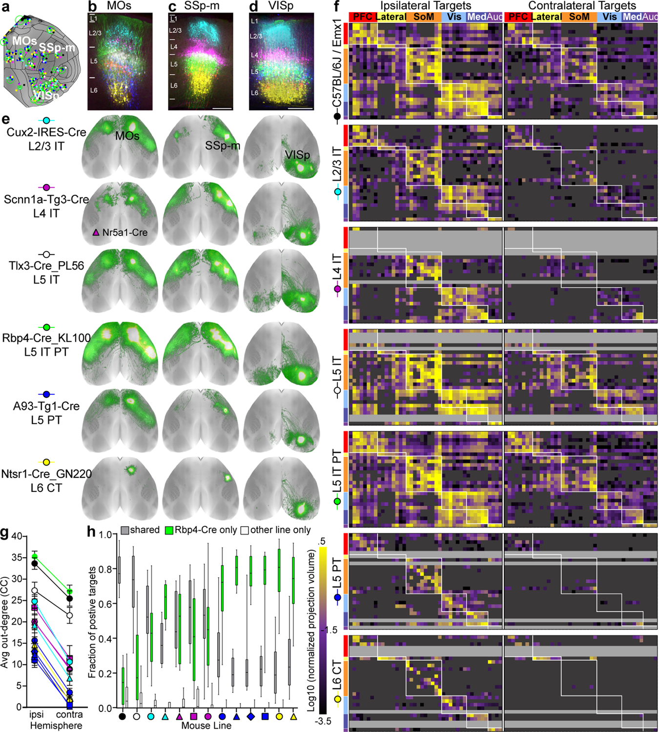
(a) 43 groups of experiments spatially-matched to one Rbp4 anchor (green dots). Most group members were < 500 μm from the anchor (median = 296 μm). Green circles indicate the variance in distance to Rbp4 for each group. (b-e) Data from three groups are shown. (b-d) STPT images at the center of each injection site per Cre line were manually overlaid by finding the best match between the pial surface (top) and white matter boundary (bottom), then pseudocolored by line. Scale bar = 250 μm. (e) Top down views of CC projections for spatially-matched experiments. (f) Directed, weighted connectivity matrices (27 × 86) for seven mouse lines: WT and the six Cre lines in (e). Each row contains the log10-transformed normalized projection volumes (NPV) from a single experiment in one of 27 source areas. Columns show cortical target regions. Rows and columns follow the same order in each matrix. White boxes highlight regions in the same module. True negatives and passing fibers were masked out (dark grey). Rows for which an experiment was missing (often because of low Cre expression) are light grey. The color map ranges from 10−3.5 to 100.5 Log NPV. It is truncated at both ends. (g) Average out-degrees (+/− SEM) across all sources for each Cre line are plotted for ipsilateral and contralateral cortex. (h) The fraction of true positive targets shared by each line with its Rbp4 anchor is shown in the box plot (gray). The fraction of positive targets unique to Rbp4 (green) or to the line indicated (white) are also shown. Box plots show median and IQR. Whiskers show min and max values.
To quantitatively compare across Cre lines, we first manually identified true positive and negative connections for each experiment in the anchor groups (43 ipsilateral and 43 contralateral targets in 364 experiments = 31,304 connections checked, Supplementary Table 4). We noted when a target contained only fibers of passage, and considered it a true negative. Using automated segmentation and registration to CCFv3, we generated a weighted connectivity matrix (using normalized projection volume, NPV, Methods) for each Cre line (WT and Emx1 were merged, Extended Data Fig. 1e–g), and applied the true positive mask to remove true negative connections (Fig. 2f). We selected only one anchor group per cortical region for visualization if there was a significant, positive correlation between Rbp4 replicates (Spearman r >0.8), resulting in 27 groups; 25 unique areas and two locations in MOs and SSs.
Overall, the CC matrices reveal several features of layer/class-specific connectivity in terms of number and specificity of connections. The average “out-degree” (number of targets, Fig. 2g) from Rbp4 is larger in both hemispheres compared to every other Cre line, except for Tlx3 on the contralateral side. L5 PT and L6 CT lines had the fewest targets in both hemispheres, followed by the L2/3, L4, and L5 IT lines. For every line, there are fewer (or no) contralateral compared to ipsilateral connections.
We determined how much overlap exists between the specific set of cortical targets contacted in each experiment and its Rbp4 anchor (Fig. 2h). WT/Emx1 projections went to ~80% of the same targets as Rbp4 axons. A roughly equal number of targets were unique to either WT or Emx1 (12.7%, 7%) perhaps due to injection variability or different viral tracers. For every other Cre line, essentially all projections went to a subset of L5 Rbp4 targets (Fig. 2h, <5% of targets unique to any line). Within L5, IT cells have the most overlap with Rbp4 targets, while PT cells have the least (Fig. 2e,f). Fewer projections to the contralateral hemisphere from L2/3 account for most of the differences with L5 (Fig. 2g).
Thalamocortical projections by source/class
To investigate TC connections, we selected 81 out of 254 injection experiments in WT and Cre driver lines based on the extent of anatomical restriction to a single region. These experiments cover 29 out of 44 thalamic nuclei in CCFv3 (Supplementary Tables 1, 2, Extended Data Fig. 5a). Most thalamic nuclei known to contain cortical projection neurons are included, except for PoT, SGN, AD, and IAM23.
We visually inspected the brain-wide axonal projection patterns and classified these 81 experiments based on previous definitions for Core, Matrix and Intralaminar TC projection classes18,23. Each experiment was manually assigned to one of four groups, or “none” if no TC axons were observed (Fig. 3a); (1) Core: labeled axons were observed in a small number of cortical targets with axons predominantly ramifying in L4, (2) Intralaminar: labeled axons were predominantly observed in the striatum, with weak or diffuse cortical axons present, (3) Matrix (focal): labeled axons targeted L1 in a small number of nearby targets, and (4) Matrix (multiareal): labeled axons targeted L1 in a more distributed set of targets. Most thalamic nuclei could be assigned to one class, although this does not preclude regions having mixed classes (Fig. 3b, Supplementary Table 1). Only three regions were assigned “core” type projections; the primary sensory thalamic nuclei, VPL, VPM, and LGd19,21. Most thalamic sources were matrix or intralaminar.
Figure 3. Thalamocortical projection patterns by region and class.
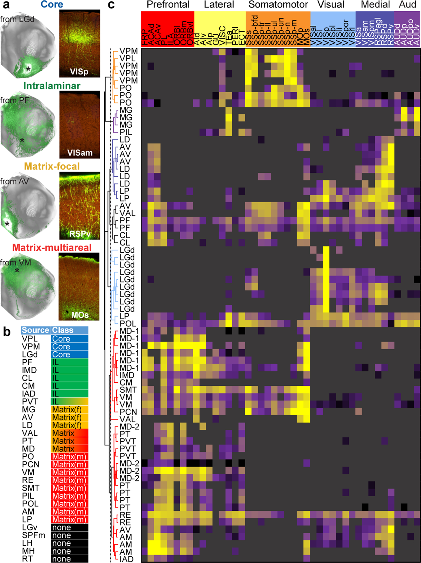
(a) Left, flat map views show TC projections labeled from the region indicated. Right, STPT images from the center of a cortical target (* on left) show example axon lamination patterns associated with each projection class. (b) Key summarizes projection class assigned for 29 thalamic nuclei. (c) The TC connectivity matrix (70 × 43) for individual viral tracer injection experiments with verified cortical projections. Each row shows log10-transformed NPVs from one experiment to the 43 ipsilateral cortical targets (columns). Cre line names for each row are in Supplementary Table 5). Unsupervised hierarchical clustering, using Spearman correlation and average linkages, revealed 7 clusters containing thalamic regions with cortical projection patterns resembling the cortical modules. Matrix color map is identical to Fig. 2.
Unlike the cortex, which is organized into distinct projection classes within layers of a single region, thalamic nuclei contain relatively homogenous populations of cortically-projecting neurons34. Since we used multiple Cre lines and WT mice for thalamic injections (Supplementary Table 1), we generated a TC connectivity matrix to compare patterns of individual experiments (Fig. 3f). We manually identified true positive and true negative (including fibers of passage) connections for cortical targets (43 ipsilateral and 43 contralateral targets in 81 experiments = 6,966 connections manually checked, Supplementary Table 5), and performed hierarchical clustering on the masked weights (Fig. 3c). Most sources with multiple injections clustered together, even those from different lines. Exceptions included MD, where further analyses showed that precise location mattered more than Cre line (MD-1 experiments are in mid-to-caudal MD, MD-2 experiments are in the rostral portion). The specific patterns of cortical areas targeted by each cluster of thalamic nuclei were remarkably like the cortical modules defined by CC connections (Extended Data Fig. 5b).
Corticothalamic projections by layer/class
We also used the Rbp4 anchored cortical experiments to generate weighted CT connectivity matrices. We again identified true positive and true negative connections, this time for all thalamic targets (44 ipsilateral and 44 contralateral targets in 256 experiments = 22,528 CT connections manually checked, Supplementary Table 6). As expected based on previous literature, most cortical projections to the thalamus were observed from L5 PT and L6 CT Cre lines (and WT), with minimal to no true positive connections from L2/3, L4, and L5 IT lines (Supplementary Table 6). We focused our subsequent analyses on Rbp4 to represent L5 PT, given its more comprehensive coverage. Connection strengths were significantly correlated between L6 CT lines Ntsr1 and Syt6 (Fig. 4d), so we averaged or merged these data (Fig. 4b).
Figure 4. Corticothalamic projections from layers 5 and 6.
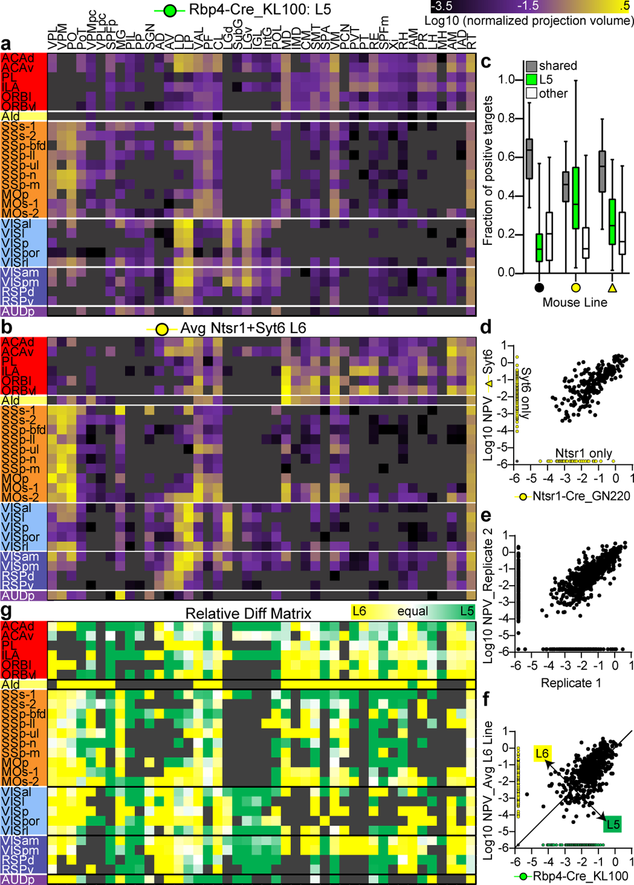
(a,b) CT connectivity matrices (27 × 44) for L5 (a, Rbp4) and L6 (b, average of Ntsr1 and Syt6). Each row shows log10-transformed NPVs from one of the 27 cortical source areas in Fig. 2 to the 44 ipsilateral thalamic target regions (columns). (c) The fraction of true positive CT targets shared by WT (black circle) and each L6 line (yellow) with its Rbp4 anchor is plotted in the box plot (gray). The fraction of positive targets unique to Rbp4 (green) or unique to the L6 line (white) are also shown. Box plots show median and IQR. Whiskers show min and max values. (d) Log NPVs for thalamic targets shared by Ntsr1 and Syt6 were significantly correlated (Spearman r=0.77, p<0.0001). (e) Log NPVs for thalamic targets shared by replicate experiments in the same Cre line < 500 μm apart were significantly correlated (Spearman r=0.84, p<0.0001). (f) The average log NPVs originating from L6 are plotted against L5 for all spatially-matched experiments (Spearman r=0.65, p<0.0001). (g) The matrix shows the relative difference for each source x target connection originating from L5 vs. L6 (L5−L6/L5+L6).
L5 and L6 CT matrices appear similar, but have quantitative differences (Fig. 4a,b). Many thalamic targets receive inputs from both layers (Fig. 4c), and the connection weights for shared targets is significantly correlated (Fig. 4f). However, this coefficient is smaller than that between replicate experiments (Fig. 4e) and between the L6 lines (Fig. 4d). We calculated and visualized relative differences in input strength from L5 and L6 for every source-target pair in the anchor group matrix (Fig. 4g). Some targets are contacted more, or less, by L5 or L6 depending on source region, but other targets have stronger L5 or L6 input regardless of source (i.e., bands of a single color down a column in Fig. 4g).
Notably, some CT projections clearly travel through thalamic regions before reaching their final targets, but also form synapses in those areas. Although entire regions containing only passing fibers were masked out, remaining connections can contain a mix of fibers and terminals. To determine the impact this kind of axonal trajectory has on quantification of CT connection strengths, we compared a subset of spatially-matched datasets in L5 and L6 Cre lines using sypEGFP to preferentially label terminals over fibers (Extended Data Fig. 6, Methods). We report a strong linear relationship between measured connection strengths, and between L5/L6 relative differences with these two tracers, showing that EGFP tracer results can be used confidently for quantitative estimates of CT strengths. Nevertheless, this is an important consideration, as across the entire brain connection strengths from sypEGFP experiments are on average lower than EGFP (Extended Data Fig. 1c), specifically by ~0.5 log units for Rbp4 CT targets (Extended Data Fig. 6k).
Laminar termination patterns in cortex
Using automated image registration to CCFv3, we quantified projection strengths by layer within each cortical target (registration precision in Extended Data Fig. 7a–c, Supplementary Table 7, Methods). Then, to identify common laminar termination patterns across all sources and lines, we performed unsupervised hierarchical clustering with the complete dataset (849 cortical and 81 thalamic experiments). Data had to pass three filters: (1) target connection strength (log10-transformed NPV) was >−1.5. This threshold was chosen after analyzing NPV frequency distributions for a set of manually-verified true positive and true negative connections (Extended Data Fig. 7d). (2) Percentage of infection volume in the primary source was >50%, and (3) self-to-self (within area) projections were removed. Following these steps, if present, multiple experiments were averaged, resulting in a total of 7,063 (660 thalamus, 6,403 cortex) unique source-line-target connections (Supplementary Table 8). We identified nine clusters (Fig. 5a). The median relative density values for each layer and the overall frequencies of these clusters are shown in Fig. 5b–d. Representative images from specific connections (a given source-line-target) assigned to each cluster from a cortical and thalamic source are shown in Fig. 5e.
Figure 5. Corticocortical and thalamocortical target lamination patterns.

(a) Unsupervised hierarchical clustering on relative projection density per layer. Each column is a unique combination of mouse line, cortical or thalamic source area, and cortical target. Connections to agranular (no L4) regions are colored gray for L4. The dotted line indicates where the dendrogram was cut into 9 clusters. (b) Median relative density by layer for each cluster. (c) Number of cortical or thalamic connections in each cluster, plotted on the left and right y-axis, respectively. (d) The frequency of cortical and thalamic targets assigned to each cluster. The dotted line indicates the overall frequency of CC targets in the entire dataset (90.53%). (e) Representative STPT images show axonal lamination patterns from a connection assigned to each cluster from cortex or thalamus. In panels 4, 8, and 9, thalamic axons passing through superficial corpus callosum are indicated (*cc). (f) The relative frequency with which each cortical Cre line and TC projection class appears in the clusters. The fraction of experiments in a cluster belonging to each Cre line/class was divided by the overall frequency of experiments from that Cre line/class. A relative frequency value of “1” (white) indicates that Cre line appeared in that cluster with the same frequency as in the entire dataset. Values <1 (green) indicate lower and >1 (pink) indicate higher than expected frequency in a cluster. Dots indicate significant positive enrichment in that cluster (Fisher’s exact test, p<0.0001). (g) Schematic diagram shows significantly enriched axon lamination patterns associated with each layer and/or class of origin in the source area.
A summary of cluster representation shows that each cortical Cre line and TC projection class is associated with more than one type of target layer pattern (Fig. 5f). The most common, and significantly enriched, laminar patterns from each are schematized in Fig. 5g. L2/3 and L4 (Nr5a1) neurons project predominantly to middle layers (L2/3, L4, and L5), avoiding L1. Other L4 neurons project to L1 and either L2/3 or L5, avoiding L4 and L6. In L5, when both IT and PT classes are labeled, as in the Rbp4 line, projections target L6 and either L1 or L2/3. L5 IT neurons predominantly target superficial layers (L1 and L2/3). L5 PT neurons target either deep layers only (L5 and L6) or deep layers and L1, consistent with the L5 Rbp4-patterns representing both IT and PT patterns. L6 CT neurons project predominantly to deep layers. From thalamic sources, core neurons project to L4 and either L5 or L6, intralaminar and matrix-focal preferentially project to L5 and L6, whereas the connections coming from matrix-multiareal sources all project to L1, with differing proportions in other layers.
Hierarchy of cortical and thalamic areas
We hypothesized that the above anatomical rules could be used across all cortical and thalamic regions to build a testable hierarchical model predicting direction of information flow. We used cortical Cre line experiments (Fig. 6) because they allow incorporation of the specific layer termination patterns related to cell class, but results are also provided using WT data (Extended Data Fig. 10).
Figure 6. A hierarchical organization of areas and modules.

(a) Direction mapping results for CC and TC terminal layer patterns. Median relative density by layer for each cluster shown from Fig. 5b. (b) Direction mapping for CT connections. Scatterplot shows the log10-transformed NPV for every CT connection from L5 and L6. Points are color coded by the mapping (FF or FB) predicted from the CC+TC hierarchy. Linear discriminant analysis (red line) assigned connections below = FF and above = FB. (c) Global hierarchy scores for CC connections only (green), compared to the scores when TC and CT connections are sequentially included (pink, blue). Scores for the original, observed, data are shown as single outlined bars. Distributions of hierarchy scores were obtained from shuffled datasets (n=100). The medians of the shuffled distributions estimate the lower bound (0.001, 0.044, −0.002). (d) 37 cortical areas and 24 thalamic nuclei rank ordered by their CC+TC+CT hierarchy scores. Scores for each area using only CC or CC+TC connections are also plotted. Y-axis labels are color coded by module assignment for cortical areas. (e) Network diagram showing interconnections of all cortical visual areas (visual module = light blue, medial module = dark blue). Edge width = relative connection density (from Fig. 1e). The curved lines show outputs (left) and inputs (right) to each node. Nodes are positioned along a single axis based on hierarchical score. (f) Intermodule network diagram. Edge width = sum of connection densities from Fig. 1e.
We used an unbiased approach to identify the most optimal label for each of the nine clusters; feedforward (FF) or feedback (FB). We defined an initial hierarchical position for each cortical area (as both a source and target) using the averaged difference of FB and FF connections, normalized by a confidence measure for each cortical Cre line (Eqs 2, 3, 4 in Methods, see also results without this confidence term in Extended Data Fig. 10). We searched over all possible mappings between the nine layer patterns and directional assignments, and determined which mapping resulted in the most self-consistent initial hierarchy (i.e., maximized the global hierarchy score, which measures how consistent the obtained hierarchy is with directions of individual connections, Eq 5 in Methods). For CC connections, clusters 2, 6, and 9 were assigned to one direction, and 1, 3, 4, 5, 7 and 8 to the other (Fig. 6a). For TC projections, clusters 2 and 6 were assigned the same direction and the rest in the other (Eqs 7–9 in Methods). Cluster 9 switched directions for CC and TC. We confidently labeled these two directions as either FF or FB based on extensive anatomical analyses relating our observed layer patterns to known hierarchical order and rules between reciprocally connected regions (Extended Data Fig. 8,9)35–38. After obtaining initial hierarchy positions with the most optimal mappings, scores were iterated to further refine the hierarchy (Eqs 6-1, 6-2, 10-1, 10-2 in Methods).
To label CT connections we used the Cre-defined L5 and L6 projection strengths (thresholded by Log10-transformed NPV >−2.5, Extended Data Fig. 7e, Eq 11 in Methods). Linear Discriminant Analysis was applied to assign CT connections into FF or FB classes most self-consistent with the direction predicted from a CT hierarchy constructed first from CC and TC projections (Fig. 6b, Eq 12 in Methods, Supplementary Table 9).
Using these rules, we obtained three versions of hierarchy based on (1) CC connections only, (2) CC and TC connections, and (3) CC, TC, and CT connections. We demonstrate that there is significant hierarchical organization by comparing global hierarchy scores with corresponding distributions of scores from shuffled connections (Fig. 6c, Extended Data Fig. 10f). Adding thalamus connections essentially doubled the hierarchy scores (0.069, 0.120, and 0.128, CC, CC+TC, CC+TC+CT respectively). Nonetheless, by comparing the global hierarchy scores with their maximums (0.679, 0.636, and 0.683, Methods), it appears to be a rather shallow hierarchy.
Final hierarchical positions for 37 cortical areas and 24 thalamic nuclei are presented in Fig. 6d (Supplementary Table 9). Most thalamic regions are located at the bottom or top, suggesting pure driver or modulator effects on the cortical areas with which they are connected. Several thalamic nuclei appear mid-hierarchy, indicating more balanced numbers of FF and FB connections. For cortical regions, primary visual cortex is at the bottom and the prefrontal area ORBvl is at the top. Predicted hierarchical positions were broadly similar across the three versions (CC, CC+TC, or CC+TC+CT). Most regions had only minor shifts in position. The largest shifts occurred in thalamic regions when adding CT connections. Hierarchies were also exceedingly robust to contributions from any single Cre line or layer/projection class (Extended Data Fig. 10h).
Similar methods were applied to predict hierarchy for subsets of areas (visual cortex, Fig. 6e) and between modules (Fig. 6f). The intermodule hierarchy had a relatively low global score (0.07) compared to the all-area hierarchy (0.13), but it was more obviously organized into distinct levels; primary sensory modules at the bottom, lateral and medial modules in the middle, and prefrontal at the top.
Discussion
We used a genetic viral tracing approach, building on our previously established whole brain imaging and informatics pipeline, to map projections originating from unique cell populations in the same cortical area, and from distinct projection classes in the thalamus. Our study represents a big step toward a true mesoscale connectome39. It will be informative for future connectome studies with more refined cell types and single cells40–42, which will no doubt reveal additional principles of cell type-specific brain connectivity43. With these mesoscale data, we derived several generalizable anatomical rules of cortical and thalamic connections, and tested whether the organizing principle of a hierarchy applies to mouse cortex and thalamus.
The cortex is organized as a modular network3,9,11, which provides a structural view of possible paths of information flow, but does not impose direction or order onto that flow. In contrast, a hierarchy implies that interareal connections belong to at least two general types: feedforward or feedback. Specific anatomical projection patterns were previously associated with carrying information in these directions in primate and rodent visual cortex12,13,36,38. In our data, we observed many similar patterns. Two patterns that differed were the superficial layer projections (cluster 1) and the deep layer projections (cluster 9). Felleman and van Essen (1991) noted the occasional superficial only pattern, but they called it feedback because it did not involve L4. Our results suggest this pattern is associated with feedforward. The strength and presence of projections between areas from the predominantly L4 Cre lines was also unexpected given canonical circuit diagrams44, and might be explained by varying degrees of layer selectivity. However, by reconstructing the complete dendritic and axonal morphology of single cells, we directly show that L4 neurons, even spiny stellate cells, can in fact have long-range projections.
The hierarchy that we find is shallower than one might have expected, even with inclusion of thalamic regions. The difference between the lowest and the highest areas is less than two full levels, and the all-area hierarchy global score is at 19% between random and perfectly hierarchical. This might be characteristic of the mouse cortex given its high connection density, particularly when considering all non-zero connection strengths45. We did not explicitly include strengths in computing hierarchy, except that weak connections were removed. Notably, hierarchical position alone does not explain all the connections of a given area. This complexity may be why some have argued the concept of a hierarchy is “overly simplistic” for describing functional properties46. Given the number of different connection types arising from a single area, future computational models incorporating more than feedforward and feedback labels will enable novel insights into organization of brain networks.
Cortical hierarchies were previously derived from classic anterograde or retrograde tracing without cell class resolution. Using Cre lines, we mapped both layer of origin and target lamination pattern in the same experiment. We found L2/3 and L4 neurons have predominantly feedforward layer projection patterns, while L5 and L6 neurons have both feedforward and feedback. However, these general relationships are dependent on the specific source-target connection and Cre line. The Cre dataset, with all this detail, indeed produced the most robust hierarchy (Extended Data Fig. 10f). However, our results from wild type mice provide a solid benchmark for others interested in applying these hierarchical model algorithms on classic tracing data. Calculating global hierarchy scores for other datasets will enable direct comparisons between species, and quantitative assessments of how development or disease might impact hierarchical organization.
Methods
Mice
Experiments involving mice were approved by the Institutional Animal Care and Use Committees of the Allen Institute for Brain Science in accordance with NIH guidelines. Sources of mouse lines are listed in Supplementary Table 1. Characterization of transgene expression patterns in many Cre driver lines used in this study were previously described26 and available through the Transgenic Characterization data portal (http://connectivity.brain-map.org/transgenic). Cre lines were originally derived on various backgrounds, but the majority were crossed to C57BL/6J mice > 10 generations and maintained as heterozygous lines upon arrival. Tracer injections were performed in male and female mice at an average age of P56 + 10 days. Mice were group-housed in a 12-hour light/dark cycle. Food and water were provided ad libitum.
Tracers and injection methods
rAAV was used as an anterograde tracer. For most regions, stereotaxic coordinates were used to identify the appropriate location for a tracer injection. Atlas-derived stereotaxic coordinates were chosen for each target area based on The Mouse Brain in Stereotaxic Coordinates47. Anterior/posterior (AP) coordinates are referenced from Bregma, medial/lateral (ML) coordinates are distance from midline at Bregma, and dorsal/ventral (DV) depth is measured from the pial surface of the brain. Stereotaxic coordinates used for each experiment can be found through the data portal. For a subset of experiments in the left hemisphere, we first functionally mapped the visual cortex using intrinsic signal imaging (ISI) through the skull, described below to assist in targeting injections. A pan-neuronal AAV expressing EGFP (rAAV2/1.hSynapsin.EGFP.WPRE.bGH, Penn Vector Core, AV-1-PV1696, Addgene ID 105539) was used for injections into wildtype C57BL/6J mice (stock no. 00064, The Jackson Laboratory). To label genetically-defined populations of neurons, we used either a Cre-dependent AAV vector that robustly expresses EGFP within the cytoplasm of Cre-expressing infected neurons (AAV2/1.pCAG.FLEX.EGFP.WPRE.bGH, Penn Vector Core, AV-1-ALL854, Addgene ID 51502) or, a Cre-dependent AAV virus expressing a synaptophysin-EGFP fusion protein to more specifically label presynaptic terminals (AAV2/1.pCAG.FLEX.sypEGFP.WPRE.bGH, Penn Vector Core).
Functional mapping of visual field space by intrinsic signal optical imaging (ISI) was used in some cases to guide injection placement. Additional details of this procedure can be found online (http://help.brain-map.org/display/mouseconnectivity/Documentation?preview=/2818171/10813533/Connectivity_Overview.pdf). Briefly, a custom 3D-printed headframe was attached to the skull, centered at 3.1 mm lateral and 1.3 mm anterior to Lambda on the left hemisphere. A transcranial window was made by securing a 7-mm glass coverslip onto the skull in the center of the headframe well. Mice were recovered for at least seven days before ISI mapping. ISI was then used to measure the hemodynamic response to visual stimulation across the entire field of view of a lightly anesthetized, head-fixed, mouse. The visual stimulus consisted of sweeping a bar containing a flickering black-and-white checkerboard pattern across a grey background48. To generate a map, the bar was swept across the screen ten times in each of the four cardinal directions, moving at 9° per second. Processing of sign maps followed methods previously described49, with minor modifications. Phase maps were generated by calculating the phase angle of the pre-processed Discrete Fourier Transform at the stimulus frequency. The phase maps were used to translate the location of a visual stimulus displayed on the retina to a spatial location on the cortex. A sign map was produced from the phase maps by taking the sign of the angle between the altitude and azimuth map gradients. Averaged sign maps were produced from a minimum of three time series images, for a combined minimum average of 30 stimulus sweeps in each direction. Visual area segmentation and identification was obtained by converting the visual field map to a binary image using a manually-defined threshold and further processing the initial visual areas with split/merge routine49. Sign maps were curated and the experiment repeated if; (1) <6 visual areas were positively identified, (2) retinotopic metrics of VISp were out of bounds (azimuth coverage within 60–100 degrees and altitude coverage within 35–60 degrees) or, (3) auto-segmented maps needed to be annotated with more than 3 adjustments. Each animal had 3 attempts to get a passing map.
ISI images were acquired using a pair of Nikon lenses (Nikkor 135 mm f/2.8 lens and 50 mm f/1.8), providing a magnification of 2.7x. Illumination was from a ring of sequential and independent LED lights, with green (peak wavelength of 527 nm and FWHM of 50 nm; Cree Inc., C503B-GCN-CY0CO791) and red spectra (peak wavelength of 635 nm and FWHM of 20 nm; Avago Technologies, HLMP-EG08-Y2000), via a bandpass filter (630/92 nm, Semrock, FF01), and acquired with a sCMOS camera (Andor, Zyla 5.5 10-tap). Illumination and image acquisition were controlled with an in-house GUI software written in Python. An image of the surface vasculature was acquired with green LED illumination to provide fiduciary marker references on the surface of the brain.
All mice received one unilateral injection into a single target region. For injections using stereotaxic coordinates from Bregma as a registration point, procedures were followed as previously described1. For ISI-guided injections, the glass coverslip of the transcranial window was removed by drilling around the edges and a small burr hole drilled, first through the Metabond and then through the skull using surface vasculature fiducials obtained from the ISI session as a guide. An overlay of the sign map over the vasculature fiducials was used to identify the target injection site. rAAV was delivered by iontophoresis with current settings of 3 μA at 7 s ‘on’ and 7 s ‘off’ cycles for 5 min total, using glass pipettes (inner tip diameters of 10–20 μm).
Some injections were done into lines with regulatable versions of Cre. Tamoxifen-inducible Cre line (CreER) mice were treated with 0.2 mg/g body weight of tamoxifen solution in corn oil via oral gavage once per day for 5 consecutive days starting the week following virus injection. Trimethoprim-inducible Cre line (dCre), mice were treated with 0.3 mg/g body weight of trimethoprim solution in 10% DMSO via oral gavage once per day for 3 consecutive days starting the week following virus injection. For these Cre lines, brains were collected 4 weeks from the rAAV injection date as opposed to 3 weeks. All mice were deeply anesthetized before intracardial perfusion, brain dissection, and tissue preparation for serial imaging as previously described1.
Serial two-photon tomography and image data processing
Imaging by serial two-photon tomography (STPT, TissueCyte 1000, TissueVision Inc. Somerville, MA) has been described1,50, and here we used the exact same procedures as our earlier published studies1,51. In brief, following tracer injections, brains were imaged using STPT at high x-y resolution (0.35 μm × 0.35 μm) every 100 μm along the rostrocaudal z-axis, after which the images underwent QC and manual annotation of injection sites, followed by signal detection and registration to the Allen Mouse Brain Common Coordinate Framework, version 3 (CCFv3) through our informatics data pipeline (IDP).
The IDP manages the processing and organization of the image and quantified data for analysis and display in the web application as previously described1,52. The two key algorithms are signal detection and image registration. Previous methods were implemented, except that two variations of the segmentation algorithm were employed, depending on the virus used for that experiment; one was tuned for EGFP, and one for SypEGFP detection. High-threshold edge information was combined with spatial distance-conditioned low-threshold edge results to form candidate signal object sets. The candidate objects were then filtered based on their morphological attributes such as length and area using connected component labelling. For the SypEGFP data, filters were tuned to detect smaller objects (punctate terminal boutons vs long fibers). In addition, high intensity pixels near the detected objects were included into the signal pixel set. Detected objects near hyper-intense artifacts occurring in multiple channels were removed. We developed an additional filtering step using a supervised decision tree classifier to filter out surface segmentation artifacts, based on morphological measurements, location context and the normalized intensities of all three channels.
The output is a full resolution mask that classifies each 0.35 μm × 0.35 μm pixel as either signal or background. An isotropic 3D summary of each brain is constructed by dividing each image series into 10 μm × 10 μm × 10 μm grid voxels. Total signal is computed for each voxel by summing the number of signal-positive pixels in that voxel. Each image stack is registered in a multi-step process using both global affine and local deformable registration to the 3D Allen mouse brain reference atlas as previously described52. Segmentation and registration results are combined to quantify signal for each voxel in the reference space and for each structure in the reference atlas ontology by combining voxels from the same structure.
Once an image series passes quality control steps, injection site polygons are manually drawn overlaying the cell bodies of infected neurons. These polygons are informatically warped into the CCFv3 atlas space. Green channel signal intensity within the polygons was used to identify which structures have been injected, and to quantify the relative magnitude of their infections. The structure receiving the largest proportion of signal intensity was identified as the primary injection site structure, and all other structures were considered secondary structures containing infected cells. A quantified injection summary is provided for each image series through the data portal that shows the relative amounts of signal detected within each infected structure.
Quantification of projection strengths using segmentation and registration
Projection signals can be quantified in several ways using our informatics pipeline (see SDK help: https://allensdk.readthedocs.io/en/latest/connectivity.html#structure-level-projection-data). Here, we most frequently report “normalized projection volume”, which is the volume of detected projection signals in all voxels in a structure (in mm3), divided by the total volume of detected signal in the manually annotated injection site. We also use the “normalized connection densities” output from the voxel-level interpolation model for modularity analyses in Fig. 1e. Connection density is the sum of detected projection pixels divided by the sum of all pixels in that voxel or structure. Normalized connection density is this value divided by the injection site density.
It is very important to note that even after undergoing our QC procedures, these informatically-derived measures of connection strength can include artifacts (false positives), and, particularly for the EGFP tracer, report total signal from labeled axons, including passing fibers and synaptic terminals. For this reason, we performed extensive manual checking of all CC, CT, and TC targets to remove any signals from regions in which we could not identify any true positive axons or terminals, as described in the Results.
Morphological reconstruction of single L4 neurons.
The Cux2-IRES-CreERT2 driver line was crossed with a novel TIGRE2.0 reporter line27, Ai166, also known as TIGRE-MORF53. Briefly, Ai166 expresses a Cre-dependent MORF transgene, composed of a farnesylated EGFP preceded by a stretch of 22 Guanidine nucleotides (22G-GFPf), which puts the transgene out-of-frame. Rare DNA replication errors lead to the deletion of one G, correcting the frameshift, and leading to GFPf expression. Combining Ai166 with a CreERT2 line and giving mice a low dose of tamoxifen produces sparse cellular labeling well suited for 3D morphological reconstruction53. High resolution whole brain imaging by fluorescence microscopic optical sectioning tomography (fMOST) has been described previously54; similar protocols were used here to image the Cux2-IRES-CreERT2;Ai166 brain. Specifically, high resolution block-face fluorescence imaging was done in coronal planes. Using a diamond knife, 1.0 μm sections were removed before imaging subsequent planes. The process is repeated through the entire rostral-caudal extent of the mouse brain, producing more than 10K images with a resolution of 0.3 × 0.3 × 1 μm (XYZ). Following acquisition of the complete fMOST image stack, it was converted to a multi-level navigable dataset using the Vaa3D-TeraFly program55, then reconstructions were performed using Vaa3D-TeraVR software tools built to facilitate semi-automated and manual reconstructions56.
Creation of the cortical top-down and flattened views of the CCFv3 for data visualization.
A standard z-projection of signal in a top-down view of the cortex mixes signal from multiple areas. Visualizations of fluorescence in Figs. 1–3 instead project signal along a curved cortical coordinate system that more closely matches the columnar structure of the cortex. This coordinate system was created by first solving Laplace’s equation between pia and white matter surfaces, resulting in intermediate equi-potential surfaces. Streamlines were computed by finding orthogonal (steepest descent) paths through the equi-potential field. Cortical signal can then be projected along these streamlines for visualization.
A cortical flatmap was also constructed to enable visualization of anatomical and projection information while preserving spatial context for the entire cortex. The flatmap was created by computing the geodesic distance (the shortest path between two points on a curve surface) between every point on the cortical surface and two pairs of selected anchor points. Each pair of anchor points form one axis of the 2D embedding of the cortex into a flatmap. The 2D coordinate for each point on the cortical surface is obtained by finding the location such that the radial (circular) distance from the anchor points (in 2D) equals the geodesic distance that was computed in 3D. This procedure produces smooth mapping of the cortical surface onto a 2D plane for visualization. This embedding does not preserve area and the frontal pole and medial-posterior region is highly distorted. As such, all numerical computation is done in 3D space. Similar techniques are used for texture mapping on geometric models in the field of computer graphics57.
Network modularity analysis
The matrix of connection weights between cortical areas (Fig. 1e) was obtained from a novel model of voxel-level connectivity29. We analyzed the network structure of this graph using the Louvain Community Detection algorithm from the Brain Connectivity Toolbox (https://sites.google.com/site/bctnet/)30,58. We determined the modularity metric (Q) at various levels of granularity by varying the resolution parameter, γ, from 0–2.5 in steps of 0.1. Q quantifies the fraction of connections inside modules minus the fraction of connections expected inside the same modules if the network was connected randomly, i.e., Q=0 has no more intramodule connections than expected by chance, while Q>0 indicates a network with some community structure.
For each value of γ, the modularity was computed 1000x and each pair of regions received an affinity score between 0 and 1. The affinity score is the probability of two regions being assigned to the same module weighted by the modularity score (Q) for that iteration, thereby assigning higher weights to partitions with a higher modularity score. Each region was assigned to the module with which it had the highest affinity, with the caveat that all structures within a module had an affinity score >= 0.5 with all other members of the module. For each value of γ, we also generated a shuffled matrix containing the same weights but with the source and target regions randomized. The modularity for the cortical matrix (Q) and the shuffled matrix (Qshuffled) were evaluated at each value of γ. As stated in the results, we chose to focus on the modules identified at γ=1.3 (Q=0.36) where the difference between Q and Qshuffled was at its peak (0.22±0.017), although it should be noted that it was relatively stable between γ=1 and γ=1.8 (0.21±0.019 at γ=1, 0.20±0.012 at γ=1.8). Modules were identical from γ=1.3 to γ=1.5 and showed only minor differences for γ between 1 and 2.
Statistics and Reproducibility
We used the software program GraphPad Prism for statistical tests and generation of graphs, and the software program Gephi for visualization and layout of network diagrams59,60. The exact numbers of tracer injection experiments per mouse line and source area are shown in Supplementary Table 1, and range from n=1 to 31. Not all experiments were independently repeated because we sought to balance the need for broad coverage across Cre lines and source areas with excessive animal use. Previously, we demonstrated that an n=1 is a good predictor of connectivity strengths across multiple animals1. In this study, we also show that the correlations between brain-wide projection strengths from experiments at matched locations within the same mouse line are consistent, positive, and significant (Spearman r>0.8, p<0.0001, Extended Data Figure 1). Sample sizes for analyses presented in all figures are mostly noted in Results, and can also be found in associated Supplementary Tables. Specifics include; for Fig. 2 g,h: n=number of mice per line, for WT, Cux2, Rbp4: n=27, Syt6: n=23, A93: n=22, Tlx3, Ntsr1: n=21, Scnn1a-Tg3: n=19, Chrna2, Efr3a: n=15, Nr5a1: n=10, Sim1: n=9, Rorb: n=6, Sepw1: n=5; for Fig. 4c: n=number of mice per line, for WT, Rbp4: n=27, Syt6: n=23, and Ntsr1: n=21; for Fig. 4d: n=1,158 total CT connections, 462 are shared above threshold, for Fig. 4e: n=1892 total CT connections, 628 shared above threshold, for Fig. 4f: n=1,158 total CT connections, 495 are shared above threshold; for Fig. 5a: n=7,063 unique connections (columns). Numbers of replicate experiments per each of the 7,063 connections ranged from 1 to 53, and are listed in Supplementary Table 8; for Fig. 5f: the number of connections assigned to each cluster is plotted in Fig. 5c, and can also be found in Supplementary Table 8 (cluster 1: n=1740, cluster 2: n=366, cluster 3: n=375, cluster 4: n=228, cluster 5: n=602, cluster 6: n=2224, cluster 7: n=102, cluster 8: n=129, cluster 9: n=1297). The number of connections per cortical Cre line can also be found in Supplementary Table 8, for A93: n=375, C57Bl6/J / Emx1: n=1,431, Chrna2: n=136, Cux2: n=703, Efr3a: n=223, Nr5a1: n=251, Ntsr1: n=246, Rbp4: n=1,149, Rorb: n=185; Scnn1a-Tg3: n=263, Sepw1: n=140, Sim1: n=108, Syt6: n=150, Tlx3: n=1,043), and per thalamic projection class was, for core: n=62, matrix-focal: n=136, intralaminar: n=160, matrix-multiareal: n=302. Fig. 6b: n=385 total CT connections.
Clustering Analyses
Unsupervised hierarchical clustering was conducted with the online software, Morpheus, (https://software.broadinstitute.org/morpheus/). Log-transforms were calculated on all values after adding a small value (0.5 minimum of the true positive array elements) to avoid Log (0). Proximity between clusters was computed using average linkages with spearman rank correlations as the distance metric. Relative layer density is the fraction of the total projection signal in each layer, scaled by the relative layer volumes in that target. The clustering algorithm works agglomeratively: initially assigning each sample to its own cluster and iteratively merging the most proximal pair of clusters until finally all the clusters have been merged. To compare distances between granular and agranular samples (those that lack a L4), we used the median of the other present layers for L4.
Unsupervised discovery of hierarchy position
Following the classification of the laminar patterns in nine clusters CC and TC connections, we used an unsupervised method to simultaneously assign a direction to a cluster type and to construct a hierarchy.
We first defined hierarchy scores of cortical regions based on layer-termination patterns of corticocortical connections. First consider a mapping function MCC for corticocortical connection:
| (1) |
which maps a type of connection cluster (, where denotes the layer termination pattern of the connection from area j to area i for Cre-line T) to either feedforward (MCC = 1) or feedback (MCC = −1) type. We search over the space of possible maps to see which map produces the most self-consistent hierarchy. Since some transgenic lines have different numbers of connections in different clusters, some maps will lead to particular transgenic lines having very biased feedforward or feedback calls. Thus, we add a confidence measure (conf(T)) for each Cre line (T), which decreases the importance of the information provided by a transgenic line to the global hierarchy if the calls from that transgenic line are biased. This allows us to reduce the bias in the regions where experiments used more Cre lines which predominantly mark feedforward or feedback connections. The Cre-dependent confidence measure is defined as:
| (2) |
with a global confidence as an average over all the inter-areal connections above the threshold (10−1.5)
| (3) |
We define the initial hierarchical position of an area as:
| (4) |
The first term, , describes the average direction of connections to area i, and thus represents the hierarchical position of the area as a target. The second term, , on the other hand, represents the average direction of connections from area i, depicting the hierarchical position of the area as a source. The hierarchical position of a cortical area is the average between its hierarchical position as source and target.
To test how self-consistent a hierarchy is we define the global hierarchy score:
| (5) |
We performed an exhaustive search over all the maps MCC for the entire set of corticocortical connections, and the most self-consistent hierarchy that maximizes the global hierarchy score is obtained when connections of cluster 2,6, and 9 are of one direction and 1,3,4,5,7, and 8 are of the opposite direction. As described in Results, we conclude that clusters 2,6 and 9 are feedback connection patterns, and the other group of clusters correspond to feedforward.
The initial hierarchy score of each area i is thus obtained by computing the average direction of connections to and from the area (Eq 4) while concurrently searching for the optimal mapping of each lamination pattern to either feedforward or feedback direction, and is bounded by −1 and 1. After obtaining the initial positions in the hierarchy, the hierarchy scores of all cortical regions are iterated until the fixed points are reached, to refine the cortical hierarchy. Without iterations, the hierarchy scores only account for the number of feedforward and feedback connections each area receives or sends out. Therefore, the initial hierarchy obtained by Eq 4 alone does not account for the hierarchy positions of the target and source areas that each cortical area makes connections to, and places any two areas with the same number of feedforward and feedback connections at the same level in the hierarchy. To address this issue, we implement a two-step iterative scheme:
| (6–1) |
| (6–2) |
where n refers to iterative steps. The first part (Eq 6-1) refines the hierarchy score of area i based on the current hierarchy scores of its target and source areas. The next part (Eq 6-2) subtracts the hierarchy scores averaged over all areas to remove possible drifts. At every iteration step we also check to see if the mapping of connection clusters to feedforward or feedback connection needs to change, however it remained constant through the iterations. We found that the hierarchy scores reach the fixed points after just a few iterations (< 5), and used 20 iterations to find the final hierarchy scores of all areas. These final hierarchy scores are denoted as the hierarchy obtained by corticocortical connections.
Next, we examined whether and how the thalamocortical connections impact the cortical hierarchy, by incorporating layer termination patterns of thalamocortical connections in addition to the corticocortical connections. As in corticocortical connections, thalamocortical connections are clustered to 9 types based on their layer termination patterns. Based on the hierarchy scores of cortical regions obtained by corticocortical connections, the mapping of the lamination patterns is obtained while the hierarchical positions of thalamic areas relative to the cortical areas are found concurrently. The mapping of the thalamocortical layer termination types to directions is defined as:
| (7) |
similar to the mapping of corticocortical connections in Eq 1. Since thalamic areas are always the source in thalamocortical connections, the initial hierarchy score of each thalamic area i is defined by the average direction of connections from the area:
| (8) |
where the mapping of the lamination patterns, MTC is obtained by searching for the most self-consistent assignment that maximizes the global hierarchy score hg:
| (9) |
The parameters Nff and Nfb refer to the numbers of feedforward and feedback thalamocortical connections, respectively. The multiplier biases the optimization method to preferentially search for mappings that result in roughly equal number of feedforward and feedback connections. Without such weight on equal divide of the connections, the search algorithm decides thalamocortical connections to be always feedforward, placing all thalamic areas below cortical areas.
As with corticocortical connections, we performed an exhaustive search over all the maps MTC for the entire set of thalamocortical connections to find the most self-consistent hierarchy that maximizes the global hierarchy score. For thalamocortical connections, we found that connections of cluster 2 and 6 are of one direction and the rest of the clusters are of the opposite direction. Again, as described in Results, we conclude that clusters 2 and 6 are feedback, and the rest correspond to feedforward patterns.
Once the initial positions of the thalamic areas in the hierarchy are obtained, hierarchy scores of thalamic and cortical areas are iterated until the fixed points are reached (20 iterations), using a full mapping function MCC+TC that combines MCC and MTC for corticocortical and thalamocortical connections, respectively:
| (10-1) |
| (10-2) |
Finally, the impact of corticothalamic connections on the hierarchy is considered. Either feedforward or feedback direction is assigned to corticothalamic connections depending on the cortical layer from where the connections originate. Specifically, we classified corticothalamic connections based on the log10-transformed normalized projection volumes (NPV) from layer 5 and layer 6 of the source areas. Therefore, the mapping of corticothalamic connections is described by:
| (11) |
We first determined the predicted direction (feedforward or feedback) of each corticothalamic connection based on the hierarchy constructed from corticocortical and thalamocortical projection patterns. These directions of corticothalamic connections show mixed L5 and L6 source expressions. To classify the corticothalamic connections to either L5 vs L6-dominance and subsequently, to feedforward vs feedback, we employed Linear Discriminant Analysis (LDA) on log10-transformed NPV values of L5 and L6 lines with a prior which biases the method to yield about equal number of L5 and L6-dominant connections. The classifier assigns feedforward direction to connections with stronger L5 source NPV, and feedback direction to L6 dominant connections, using the linear separator. Once directions of corticothalamic connections are thus obtained, the mappings MCC, MTC and MCT are combined to construct a comprehensive mapping, MCC+TC+CT, of all connections among cortical and thalamic areas to directions. The initial positions of thalamic regions in the hierarchy are computed by:
| (12) |
Where MTC+CT is the mapping of all thalamocortical and corticothalamic connections. Note that the multiplier used for initial thalamic hierarchy with TC connections only (which biases thalamus to be towards the center of the hierarchy) is not needed here, due to the presence of the CT connections in the computations. However, the bias is not fully eliminated as it influenced the initial assignment of CT and TC connections types to be feedforward or feedback. The initial hierarchy scores are iterated together with hierarchy scores of cortical areas obtained from Eq 6:
| (13–1) |
| (13–2) |
In this way, we obtained three different versions of cortical hierarchy constructed from: 1) corticocortical connections only, 2) corticocortical connections + thalamocortical connections, and 3) corticocortical, thalamocortical, and corticothalamic connections.
We examined how the additional information provided by thalamocortical and corticothalamic connections impact the self-consistency of the hierarchy by comparing the global hierarchy scores of the three different versions of hierarchy. For this purpose, we compare the global hierarchy scores without any confidence or weight multiplier:
| (14) |
In addition to the hierarchy of all areas, we also constructed the intermodule hierarchy of cortical areas. We used the same mappings obtained from construction of the all-area hierarchy, to classify the lamination patterns. For intermodule hierarchy, all the connections to and from each module are used to build the hierarchy among the modules.
Global hierarchy score of shuffled connectomes and “perfectly hierarchical” connectome
To evaluate “how hierarchical” the mouse brain is, we generated shuffled connectivity data of the connection patterns, computed the global hierarchy scores, and compared the global hierarchy scores of the shuffled connectomes to that of the mouse brain connectome. The shuffled connectivity is constructed by randomly rearranging sources and targets, while preserving the projection layer patterns and the distributions of source and target areas, within each Cre line. We generated 100 versions of shuffled connectivity data, and calculated their global hierarchy scores as was done with the original connectivity data, described in the previous section. The medians of the shuffled distributions provide an estimate of the lower bound of this score (0.001, 0.044, −0.002, for CC, CC+TC, CC+TC+CT, respectively (Fig. 6c)).
We also generated connectivity data with perfectly self-consistent hierarchy, which provides the upper bound of the global hierarchy score. To do this, we assigned a direction (feedforward or feedback) for each connection in the mouse brain connectivity data, based on the final hierarchy positions of the cortical and thalamic regions. With this “true” mapping of each connection to a direction, the global hierarchy score is computed using Eq 14, producing a value of 0.679, 0.636, and 0.683, respectively for CC, CC+TC, and CC+TC+CT connections.
Therefore, comparison of global hierarchy scores allows us to evaluate how hierarchical the mouse brain is compared to the hierarchy by chance (shuffled) and the perfect hierarchy (upper bound). The global hierarchy scores with the shuffle mean subtracted and normalized by the strictly hierarchical data provides a single measure that quantifies steepness of hierarchy across arbitrarily different connectivity data.
Extended Data
Extended Data Figure 1. Similarity of connection strengths by distance, virus, hemisphere, and Emx1-IRES-Cre or C57BL/6J mice.

(a-d) Most experiments were done with the Cre-dependent rAAV tracer, rAAV2/1.pCAG.FLEX.EGFP.WPRE. A subset of left hemisphere injections had a duplicate injection of rAAV with a synaptophysin-EGFP fusion transgene in place of the cytoplasmic EGFP (rAAV2/1.pCAG.FLEX.SypEGFP.WPRE). This tracer allowed us to address whether labeling presynaptic terminals would improve accuracy of quantifying target connection strength, particularly in brain regions containing mostly fibers of passage. Data consisted of n=275 experiments (137 EGFP: 138 SypEGFP). These were matched across Cre lines and areas, and represent n=8 Cre lines and n=26 cortical areas. For pairs of spatially-matched experiments, the average projection strength (log10-transformed NPV) measured across the entire brain was lower in SypEGFP vs EGFP experiments (~ 0.8 log unit when <500 μm apart). However, brain-wide projection values were still highly and significantly correlated. Thus, we included the SypEGFP datasets when indicated for analyses of connectivity patterns from given source areas (but only in comparison with other SypEGFP datasets). (a) Spearman correlation coefficients (R) of normalized projection volumes for all possible pairs of injections (different and same tracer, all in the same Cre line) are plotted against the distance between the injection centroids. Linear regressions showed a significant negative slope (p<0.0001) with lower R as distance between injections increases. (b) R is plotted for injections within 500 μm of each other; slopes were not significantly different from zero and means were not significantly different from each other. Average and SD for each group is shown by the large symbols on the left (EGFP v EGFP: 0.81 +/− 0.056, SypEGFP v SypEGFP: 0.79 +/− 0.064, SypEGFP v EGFP: 0.79 +/− 0.071). (c) Quantitative differences in projection strengths measured between replicates with the same virus and between SypEGFP and EGFP (logNPV (EGFP)-logNPV(SypEGFP) injections, all < 500 um apart in the same Cre line (n=133 within virus and 222 between virus comparisons). Boxplots show median, IQR, min, max values, and + indicates mean. (d) Maximum intensity projections from four experiments within 500 μm of each other illustrate overall similarities between replicate injections and tracers (Spearman R is shown for each pair). Injections targeted primary visual cortex (VISp) in Emx1-IRES-Cre mice using either EGFP or SypEGFP tracers as indicated. (e-g) Injections into Emx1-IRES-Cre mice were made into visual areas on the left hemisphere, whereas all C57BL/6J mice received injections into the right hemisphere. Following registration to the CCF, which is a symmetric atlas, we identified three pairs of experiments in which the injection centroids were < 500μm apart after flipping injection site coordinates from the left to the right. Cortical projections were visually similar across both lines and hemispheres, and cortical connectivity strengths (to the 86 cortical targets) from these individual experiments (normalized projection volumes) were positively and strongly correlated as indicated (Spearman rank, r=0.877, 0.904, and 0.965). Thus, in Fig. 2 we merged the Emx1 and C57BL/6J data to represent connection strengths from all layers and classes, and in some of the “anchor” groups we used data from both left and right hemisphere injections.
Extended Data Figure 2. Characterization of cortical projection neuron classes and layer selectivity across mouse lines.

(a) Brain-wide projection patterns were visually inspected for every experiment and manually classified into one of six categories based on projections to ipsi- and contra- lateral cortex, striatum, thalamus, and midbrain/pons/medulla structures as described for IT, PT, and CT classes. (b-d) Unsupervised hierarchical clustering (using Euclidean distance and average linkage) of projection weights validates and reveals major classes of cortical projection neurons. (b) Each column of the heat map shows one of the 1,081 injection experiments. Colors in the “manual PN class” are coded as in (c) for projection class. Rows show selected major brain regions which distinguish known classes of projection neurons. Values in each cell are the fraction of total brain projection volume in the given region. The dendrogram was split into 9 clusters, with two subclusters identified post-hoc for cluster 5. The numbers of experiments per cluster were (1: n=24, 2: n=4, 3: n=204, 4: n=158, 5a: n=148, 5b: n=230, 6: n=174, 7: n=12, 8: n=16, 9: n=111. The numbers of experiments per projection class were CT: n=119, IT: n=342, IT PT: n=158, IT PT CT: n=189, local: n=100, PT: n=173. (c) The relative frequency of experiments from manually-assigned projection classes within each cluster is shown. There was significant enrichment of 1, or 2 related, classes in each cluster (dots; Fisher’s exact t-test, p<0.01). (d) Maximum intensity projections of GFP-labeled axons across the brain from one example per cluster. (e) Characterization of layer-selectivity in wild type and 14 Cre lines derived from injection experiments. Number of experiments per line is listed in Supplementary Table 1. For every injection and line, we assessed layer-selectivity based on the manually annotated injection sites. Polygons were drawn around every injection site so that, after registration to the CCF, injection volume in each layer could be informatically-derived. A layer-selectivity index was calculated for each experiment (the fraction of the total injection volume contained in each layer, scaled by the relative volume of each layer in the injection source region, because layer volumes differ by area). Plots show individual data points and the average layer selectivity index +/− 95% confidence intervals (in black) for the set of 15 mouse lines. Red lines in each Cre graph show average values from C57BL/6J experiments. Red lines in the C57BL/6J graph are averages from the Emx1-IRES-Cre experiments, which also labels cells across all layers. There is a bias toward L5 neuron infection in both C57BL/6J and Emx1-IRES-Cre, highlighting the importance of using layer selective Cre lines for better coverage of cortical outputs.
Extended Data Figure 3. Computationally removing the distance-dependence of connection weights alters the modular structure of the cortex.

To test the degree to which spatial proximity of regions affects modularity analysis, we used a power-law to fit the distance component of our ipsilateral corticocortical connectivity matrix (Knox et al., 2019). Then, we repeated our modularity analysis on the “distance-subtracted” matrix built from these residuals. (a) Weighted connectivity matrix for 43 cortical areas showing the value of the residuals from a power-law to fit the distance component. Rows are sources, columns are targets. Colors on the rows indicate distance-subtracted community structure with varying levels of resolution (γ = 0.5–1.5 on the y axis, γ = 0.8 only on the top portion of the x-axis). Columns are colored by their module affiliation in the distance-subtracted matrix above their module affiliation in the original matrix (Figure 1e). The inset in the top left corner shows the modularity metric (Q) for each level of γ, along with the Q value for a shuffled network containing the same weights. The Q values for modularity in the distance-subtracted matrix were smaller than for the original cortical matrix (e.g., 0.2754 vs 0.4638 at γ = 0.8) and the range of values for which Q was greater than Qshuffled was narrower (0.7 ≤ γ ≤ 1.7), but some modules were still present in the distance-subtracted cortical connectivity matrix. The difference between Q and Qshuffled was greatest for γ = 0.8. The first distance-subtracted module was comprised of the entire somatomotor module, most of the lateral module, and two regions from the prefrontal module. The second distance-subtracted module contained the visual, auditory, and medial modules, plus most of the prefrontal module and one region from the lateral module (temporal association area). Notably, these modules were like those reported by Rubinov et al. (2015). As γ increased past 1.0, regions began to split from the two large modules in small groups that generally did not reflect the original divisions, except for the auditory areas. (b) Diagram shows the ipsilateral cortical network in 2D using a force-directed layout algorithm. Nodes are color coded by module. Edge thickness shows residual values and edges between modules are colored as a blend of the module colors. (c) Cortical regions color-coded by their distance-subtracted community affiliation at γ = 0.8 show spatial relationships.
Extended Data Figure 4. Whole brain single neuron reconstructions reveal L4 IT projections.
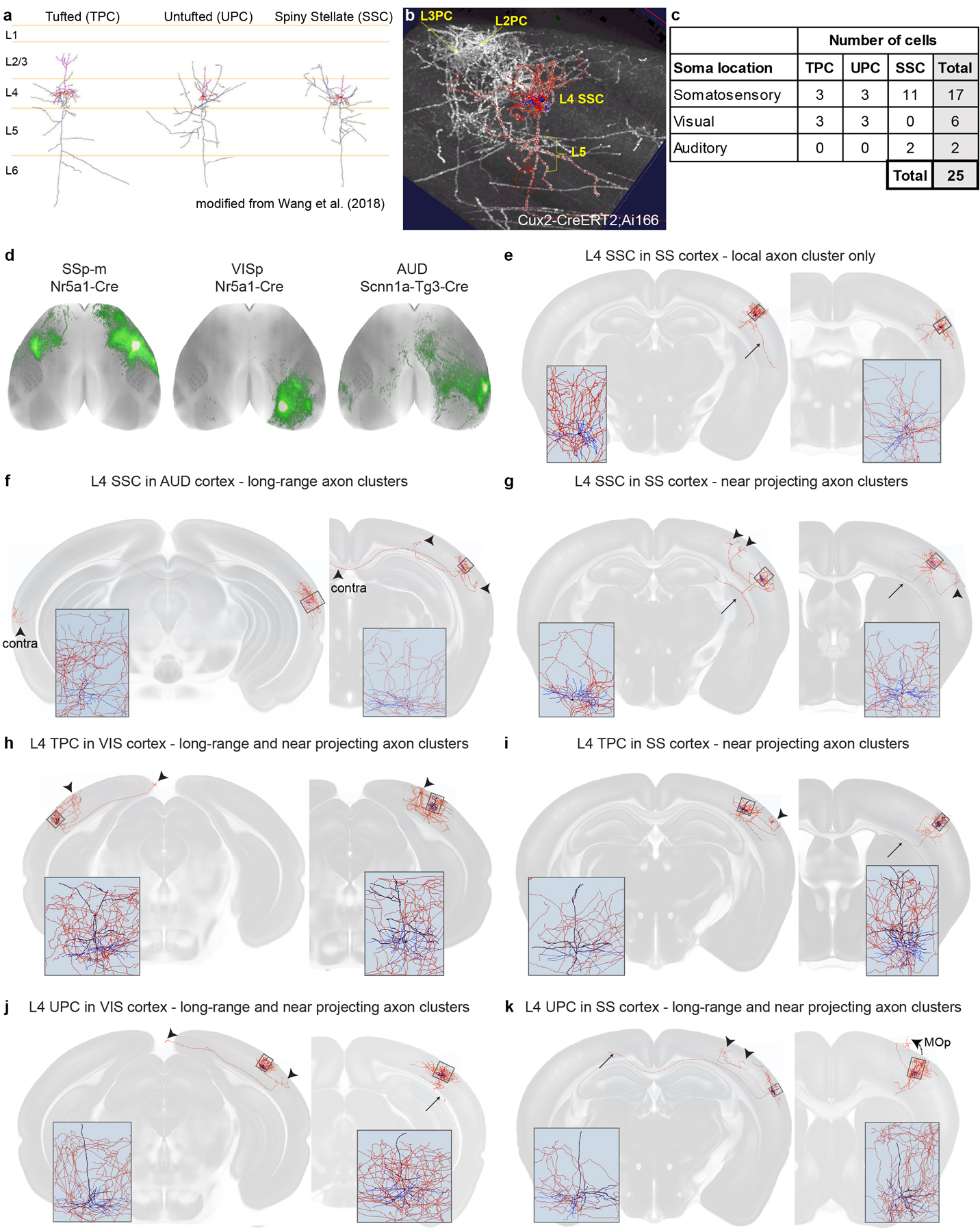
(a) L4 neurons are classified into at least 3 morphological types as shown. (b) Image shows sparse labeling of L2/3 and L4 neurons in the tamoxifen-inducible Cux2-IRES-CreERT2 driver crossed with the Ai166 reporter and using a low-dose of tamoxifen via oral gavage for 1 day. L4 neurons were identified based on their apical dendrite and local axons, using additional anatomical context when possible. Reconstruction was performed using Vaa3D-TeraVR on the high resolution whole brain image stack (composed of more than 10K images, resolution XYZ: 0.3 × 0.3 × 1 μm) acquired with a two-photon fluorescence micro-optical sectioning tomography system (2p-fMOST). (c) We identified 25 total L4 neurons for complete morphological reconstruction of dendrite and axon for three cell types and three cortical areas. In this Cre line at least, SSCs were most frequently identified. (d) Dorsal surface view shows the corticocortical projection patterns from three anterograde tracer experiments into the predominantly L4 Cre lines for somatosensory cortex (SS), visual cortex (VIS) and auditory cortex (AUD). (e-k) Each panel shows two examples of reconstructed cells of the same L4 type in SS, VIS, or AUD. Local morphology for each cell is shown in the inset. Arrowheads indicate axon clusters outside local region. Red=axon, blue=basal dendrite, black=apical dendrite. Consistent with canonical descriptions, we found SSCs in the somatosensory cortex that had only local axon clusters (e). However, even in these cases, we frequently observed what appeared as an aborted axon branch (no terminal cluster found; long arrow). We also found SSCs in SS that did have clear axon clusters in nearby areas (g), and, in AUD cortex, SSCs projected even to the opposite hemisphere (f). (h-k) Although we identified fewer TPC and UPC cell types in this experiment, for both types we still found cells with near and long-range projections.
Extended Data Figure 5. Locations and cortical projection patterns from thalamic tracer experiments.

(a) Locations of the thalamic tracer injection centroids (blue dots) are shown mapped onto virtual 2D coronal planes from the Allen CCFv3. To minimize the number of sections shown, all centroids are mapped within 200 μm of their original location. See Supplementary Table 1 (thalamus tab) for more details on Cre lines and coverage. (b) Example TC projections are shown in a flat map view of the ipsilateral cortical hemisphere for different thalamic nuclei arranged by the clusters identified in Fig. 3 and related to cortical modules. Most thalamic clusters projected primarily to a single module (Fig. 3c), but some thalamic regions projected across multiple modules (e.g., AV, VAL, PF, CL), or projected strongly to both prefrontal and another module; e.g., somatomotor (MD-1, VM), lateral (PVT, MD-2, PT) or medial regions (RE, AM).
Extended Data Figure 6. Comparison of corticothalamic projection strengths derived from EGFP and SypEGFP tracer experiments.

(a-d) Maximum intensity projections from four experiments within 500 μm of each other targeting VISp (same experiment labeled VISp-3 below) using either EGFP or SypEGFP tracers in the Rbp4-Cre_KL100 (L5) or Ntsr1_Cre_GN220 (L6) line as indicated. (a’-d’) Coronal STPT images near the center of the densest terminal zone in LGd show axon and presynaptic terminal labeling in LGd and other thalamic targets, including the ventral lateral geniculate (LGd, LGv), the intergeniculate leaflet (IGL) and the lateral posterior nucleus (LP). The anterior pretectal nucleus (APN) in the midbrain is also indicated. SypEGFP labeling is more punctate and has less fluorescence in axons and fiber tracts. (a”-d”) Coronal STPT images near the center of one of the densest terminal zones in the middle of LP. (a”’-d”’) Coronal STPT images near the center of the second densest terminal zone in the anterior part of LP. This image also contains a portion of the terminal zone in LD. (e-h) Directed, weighted, connectivity matrices (11 × 44) showing log10-transformed normalized projection volumes for the Cre lines representing CT projections labeled from Layer 5 (e,f) or Layer 6 (g,h) with EGFP or SypEGFP tracer as indicated. True negatives (including passing fibers) at the regional level were masked and colored dark grey. The color map is the same as in Fig. 4. The matrix shows relative differences for connections originating from L5 vs. L6 (L5−L6/L5+L6) for EGFP-based measures (i) and SypEGFP-based measures (j). (k) Normalized projection strengths for corticothalamic targets (n=484) were significantly correlated from matched cortical locations between EGFP and SypEGFP tracers for both Cre lines (Spearman r=0.71, 0.73, p<0.0001). On average, EGFP CT NPVs were ~ 0.5 log unit larger than SypEGFP for Rbp4 experiments, but were not different for the Ntsr1 line. (l) Normalized projection strengths for corticothalamic targets (n=484) contacted by L5 or L6 cortical neurons in matched injection locations were also significantly correlated for both EGFP and SypEGFP tracers (Spearman r=0.51, 0.60, p<0.0001), although more weakly than for the same line between viruses. Specific connections with different fiber to terminal ratios are colored by source module (light blue = from VISp, orange = from SSp, dark blue = from RSPagl). (m) Relative differences in projection strength to LP and LGd are plotted from n=6 VISp injection experiments (VISp-1 to VISp-6 in matrix rows above) for each Cre line and viral tracer. (n) Relative difference ratios calculated for L5 to L6 using EGFP are plotted against those obtained using SypEGFP (n=484 CT connections, n=278 above threshold). There is a significant correlation (Spearman r=0.68, p<0.0001). Specific connections are colored by source module (from panel l) and labeled with the target.
Extended Data Figure 7. Validation of informatics-processing steps: CCF registration and quantitation from segmentation.

(a-c) To determine how precise the registration process is which we rely on here for quantification of signal by layer in the cortex, we manually delineated layers 1 to 6b, using background fluorescence in coronal STPT images, for n=9 cortical areas (ACAd, ORBvl, AId, PERI, SSp-bfd, MOp, VISp, RSPd, and AUDp) in n=4 mice per region. We then quantified the percentage of voxels within each manually annotated layer that were assigned to all cortical layers following automated registration to the CCFv3. (a) A confusion matrix show the mean % of overlapping voxel labels averaged across these areas (individual region data in Supplementary Table 6). (b,c) Boxplots show the median and mean (indicated with “+”); whiskers show the min:max range for the % overlap for individual experiments (b) or cortical areas (c, colored dots). Across these cortical areas, the average % overlap ranged from 86–96% of voxels appropriately registered for all layers, except for L6b, which was not included in subsequent layer quantifications. For some areas and layers, the precision was worse than others, e.g., while 66% of voxels were appropriately assigned to L2/3 in ACAd, the remaining 34% were assigned to neighboring L5. In ORBvl, only 51% of voxels were appropriately labeled for L6a. We want to note, however, that delineating layer 5 from L6a in ORBvl in coronal sections using just background fluorescence was very difficult even for experienced anatomists, so some of the imprecision may in fact come from the manual drawing. Even with these exceptions noted, in all cases a large majority of voxels were registered and assigned correctly. (d-e) Frequency distributions of informatically-derived quantification for manually verified true negative and positive targets. (d) The numbers of Log10-transformed normalized projection values are plotted for all corticocortical and thalamocortical targets manually verified as true negative (n=24,272) or true positive (n=12,921). Most true positive values were between log10=−4 and log10=1. At log10=−1.5 (red arrow), 639 true negatives remained (2.6%), while 7,100 true positives were still included (54.9%), resulting in a false positive rate of 8.3% at this threshold level. (e) Numbers of Log10-transformed normalized projection values are plotted for all corticocortical and thalamocortical targets manually verified as true negative (n=15,789) or true positive (n=4,503). At log10=−2.5 (red arrow), 362 true negatives remained (2.3%), while 3,335 true positives were still included (74.1%), resulting in a false positive rate of 9.8% at this threshold level.
Extended Data Figure 8. CC projection patterns by layer and class between reciprocally connected areas with known hierarchy.

(a) In the visual module, VISp and VISal are reciprocally connected (black line). VISp is the de facto bottom of visual cortex hierarchy. The output to VISal from VISp is feedforward (FF). The reciprocal connection (VISal to VISp) is feedback (FB). In the FF direction (top), VISp projections from L2/3, L4, and L5 IT projections were densest in L2/3-L5 of VISal, and relatively sparse in L1 and L6 (cluster 4). Rbp4 projections from VISp to VISal were densest in L4 and L6, with moderate levels in L2/3 (cluster 8). L5 PT and L6 CT cells projected, albeit sparsely, to L1 and L5 (cluster 2). In the FB direction (bottom), L2/3 IT axons were broadly distributed across layers, with a sparser region in L5 (cluster 6). VISal L4 IT cells project noticeably more weakly to VISp (as opposed to the panel above), and terminate with a different pattern (L1 and L5/6, cluster 6). L5 IT cells project densely to superficial layers in VISp (cluster 1). Rbp4 axons were dense in L1 and deep layers (cluster 6). Projections from L5 PT and L6 CT cells were also sparse, but present in L1 and L6 (cluster 6). (b) In the somatomotor module, SSp-bfd and SSs cortex are reciprocally connected. SSp-bfd to SSs is FF; the reverse is FB. In the FF direction (top), L2/3 and L4 IT cells preferentially innervate L2/3-L5, with relatively fewer terminals in L1 and L6 (clusters 3 and 4). L5 IT projections densely innervate L1 and L2/3 (cluster 1). Rbp4 projections were densest in L4 and L6, with moderate levels in L2/3 (cluster 8). L5 PT and L6 CT cell projections were sparse, and to L1 and/or deep layers (cluster 2 and 6). In the FB direction (bottom), the patterns looked remarkably like FB projections from VISal to VISp. Note again the strong connection originating from L4 cells only in the FF direction. (c) VISp (in the visual module) and ACAd (in the prefrontal module) are reciprocally connected. ACAd exerts top-down control of VISp activity (FB); the reverse (VISp to ACAd) is considered FF. In the FF direction (top), L2/3, L4, and L5 cells all preferentially innervate L1 (cluster 1). In the FB direction (bottom), L2/3 cells also predominantly terminate in L1, but L5 cells project to both L1 and deep layers (L5 and L6, cluster 6). Note also there is a potentially significant sub-layer distinction; axons from VISp to ACAd are relatively deeper in L1 (or at the border of L1 and L2/3) of ACAd, compared to the more superficial termination of ACAd axons in L1 of VISp. (all panels) Overall, FF projections are more often in clusters 1, 4, and 8, and FB projections in cluster 6. Cluster assignments are indicated in each panel; n/a indicates the connection was either absent or below threshold for clustering. Areas in each module are shown in a top down cortex view and the network as a force-directed layout (edges = normalized connection density from Fig. 1e). STPT images in the approximate center of each target region show the laminar distribution of axons arising from labeled neurons in the different Cre lines. Images were rotated so that the pial surface is always at the top of each panel.
Extended Data Figure 9. TC and CT projection patterns and rules between reciprocally connected areas.

(a) Schematic summarizes observed projection patterns between core thalamic nuclei (blue circle) and their reciprocally connected cortical targets (L1–L6 color coded). Laminar patterns are from Fig. 5g. STPT images of labeled axon terminals between 3 pairs of core nuclei and primary sensory cortex that perfectly follow rules in both directions. In the FF direction (LGd to VISp, VPL to SSp-ll, VPM to SSp-n) projections are dense in L4 or L4 and L6 (clusters 4, 8). In the FB direction, CT projections predominantly arise from L6. (b) Schematic summarizes observed projection patterns between matrix-focal thalamic nuclei (orange circle) and their reciprocally connected cortical targets. STPT images of reciprocal connections between PT and ILA, MD and ORBl, and MD and AId illustrate the schematized rules. Projections from these thalamic nuclei belong to clusters with relatively less L1 axon (FF-like, clusters 3, 7, 9). The reciprocal CT input is also stronger from L6 (FB), like the core nuclei above. (c) Three schematics are shown to summarize observed projection patterns between matrix-multiareal thalamic nuclei (red circle) and their reciprocally connected cortical targets. The top schematic shows dense TC projections to L1 (FB) with CT projections originating from L5 (FF). The middle schematic (with relevant example images boxed) shows reciprocal connection patterns in which TC projections target mid-layers (FF-like) and the reciprocal CT input is stronger from L6 (FB). The bottom schematic shows the same TC projection pattern as the top schematic, but with CT projections originating ~equally from L5 and L6. STPT images show reciprocal connections between multiarea-matrix thalamic regions LP, PO, RE, and VM to 3 cortical targets each. Some regions have target-specific projections that are either FF or FB. For example, different from the LP-to-VISp projection (FB), axons from LP to VISam and ACAd target mid-layers as opposed to L1 (clusters 8 and 5, FF), and the reciprocal connection arises more from L6 (typical for FB). Projections from PO, RE, and VM to all three cortical targets are consistent with a FB projection (denser terminations in L1 and either L5 or L6 (clusters 2 and 6). Reciprocal CT projections originate from L5 or, both L5 and L6. We did not see CT input arising equally from both layers or more from L5 when the reciprocal TC projection was considered FF, consistent with the “no-strong-loops” hypothesis37. (all panels) Overall, FF projections from core thalamic regions are in clusters 4 and 8. FB from matrix-multiareal thalamic regions are in clusters 2 and 6, like CC FB. The matrix-focal results support the notion that patterns with relatively less L1 involvement (3, 5, 7, 9) are FF, particularly given the strong reciprocal input observed from L6. STPT images are from the approximate center of the axon termination field for each target region. Cortex images were rotated so that the pial surface is at the top. Cluster assignments (for TC) are indicated in each panel. Text labels above image show FF and FB direction based on relative position in Fig. 6. Dashed lines indicate region borders.
Extended Data Figure 10. Robustness of the hierarchical organization results.

We constructed multiple hierarchies using only C57BL6/J and Emx1-IRES-Cre experiments (WT) or Cre data without the Cre line confidence measure to compare with results in Fig. 6. The hierarchical position of each area and the global hierarchy score hg are defined as in Equations (4) and (5) in Methods, but with the same confidence for all lines, i.e, conf(T)=1 for all Cre lines (T). (a,b) In both cases, connection types 2 and 6 are assigned to one direction (feedback), while other clusters are grouped to the opposite direction (feedforward). Cluster 7 was not identified in the WT dataset. (c) Corticothalamic connections were also classified as in Fig. 6b for the Cre data. CT connections were not included for WT as these are exclusively defined by Cre lines. (d,e) Global hierarchy scores from the original, observed data, and the distributions of hierarchy scores obtained from shuffled datasets (n=100) are shown for CC connections only (green), compared to scores obtained when TC connections are sequentially included (pink). The upper bound scores for an artificially-perfect hierarchy using the WT datasets (e) are: 0.630 for CC and 0.601 for CC+TC connections. (f) Z-scores were calculated for the global hierarchy scores compared to shuffled data for each of the three versions of cortical hierarchy (CC, CC+TC, CC+TC+CT). The highest z-scores were observed when using Cre line confidence weighting (compared to those with no confidence weighting or wild type data only). (g) Predicted hierarchical positions of 37 cortical and 24 thalamic areas based on CC, CC+TC, or CC+TC+CT connections. Areas are ordered in each panel by the scores obtained using Cre line data with confidence weighting (Cre conf, black circles). Scores from Cre line data without confidence weighting (gray circles) and scores from wild type/Emx1-IRES-Cre data (open circles) are plotted for direct comparison. Y-axis labels are color coded by module assignment (for cortical areas). (h) Robustness of the cortical hierarchy (w/ Cre conf) against individual Cre lines and projection classes. The left panel shows Spearman rank correlation coefficients between the CC and CC+TC hierarchy with n=13 layer-/class-specific Cre lines included vs. each of the Cre lines removed. The right panel shows results when data from Cre lines with the same layer and class were removed together. Removal of these lines and classes produced relatively minor deviations from the overall hierarchy determined with all data. Note that in both panels the y-axis starts at R=0.85. For all lines and classes, the correlation with the hierarchy using the complete dataset is very high. The lowest correlations occurred following removal of Cux2-IRES-Cre, Rbp4-Cre_KL100, and Tlx3-Cre_PL56.
Supplementary Material
Acknowledgements
We thank the Animal Care, Transgenic Colony Management and Lab Animal Services teams for mouse husbandry and tissue preparation. We thank all the members of the Neurosurgery and Behavior team for viral injections, including those not listed as authors: N. Berbesque, N. Bowles, S. Cross, M. Edwards, S. Lambert, W. Liu, K. Mace, N. Mastan, C. Nayan, B. Rogers, J. Swapp, C. White, and N. Wong. We also thank H. Gu for cloning of the synaptophysin-EGFP viral vector, E. Lee, F. Griffin, and T. Nguyen for intrinsic signal imaging, and J. Royall and P. Lesnar for schematic figure preparation. This work was supported by the Allen Institute for Brain Science and, in part, by National Institutes of Health grants R01AG047589 to J.A.H, and U01MH105982 and U19EY023173 to H.Z. We thank the Allen Institute founder, Paul G. Allen, for his vision, encouragement, and support.
Footnotes
Data availability statement
Data (including high resolution images, segmentation, registration to CCFv3, and automated quantification of injection size, location, and distribution across brain structures) are available through the Allen Mouse Brain Connectivity Atlas portal (http://connectivity.brain-map.org/). Individual experiment summaries can be viewed using this link:http://connectivity.brain-map.org/projection/experiment/[insertexperimentalid]. In addition to visualization and search tools available at this site, users can download data using the Allen Brain Atlas API (http://help.brain-map.org/display/mouseconnectivity/API) and the Allen Brain Atlas Software Development Kit (SDK: http://alleninstitute.github.io/AllenSDK/connectivity.html). Through the SDK, structure and voxel-level projection data are available for download. Examples of code for common data requests are provided as part of the Mouse Connectivity Jupyter notebook to help users get started with their own analyses. Source data generated for this study are provided as Supplementary Tables as indicated throughout. Code and data files for hierarchical analyses are available through the Allen SDK and Github (https://github.com/AllenInstitute/MouseBrainHierarchy).
The authors declare no competing interests.
References
- 1.Oh SW et al. A mesoscale connectome of the mouse brain. Nature 508, 207–214 (2014). [DOI] [PMC free article] [PubMed] [Google Scholar]
- 2.Sporns O, Tononi G & Kötter R The Human Connectome: A Structural Description of the Human Brain. PLoS Comput. Biol 1, e42 (2005). [DOI] [PMC free article] [PubMed] [Google Scholar]
- 3.Zingg B et al. Neural Networks of the Mouse Neocortex. Cell 156, 1096–1111 (2014). [DOI] [PMC free article] [PubMed] [Google Scholar]
- 4.Markov NT et al. A weighted and directed interareal connectivity matrix for macaque cerebral cortex. Cereb. Cortex 24, 17–36 (2014). [DOI] [PMC free article] [PubMed] [Google Scholar]
- 5.Bota M, Sporns O & Swanson LW Architecture of the cerebral cortical association connectome underlying cognition. Proc. Natl. Acad. Sci 112, E2093–E2101 (2015). [DOI] [PMC free article] [PubMed] [Google Scholar]
- 6.Scannell JW, Blakemore C & Young MP Analysis of connectivity in the cat cerebral cortex. J. Neurosci 15, 1463–83 (1995). [DOI] [PMC free article] [PubMed] [Google Scholar]
- 7.Swanson LW, Hahn JD & Sporns O Organizing principles for the cerebral cortex network of commissural and association connections. Proc. Natl. Acad. Sci 114, E9692–E9701 (2017). [DOI] [PMC free article] [PubMed] [Google Scholar]
- 8.Bullmore E & Sporns O Complex brain networks: graph theoretical analysis of structural and functional systems. Nat. Rev. Neurosci 10, 186–198 (2009). [DOI] [PubMed] [Google Scholar]
- 9.Rubinov M, Ypma RJF, Watson C & Bullmore ET Wiring cost and topological participation of the mouse brain connectome. Proc. Natl. Acad. Sci 112, 10032–10037 (2015). [DOI] [PMC free article] [PubMed] [Google Scholar]
- 10.Wang Q, Sporns O & Burkhalter A Network analysis of corticocortical connections reveals ventral and dorsal processing streams in mouse visual cortex. J. Neurosci 32, 4386–99 (2012). [DOI] [PMC free article] [PubMed] [Google Scholar]
- 11.Swanson LW, Hahn JD, Jeub LGS, Fortunato S & Sporns O Subsystem organization of axonal connections within and between the right and left cerebral cortex and cerebral nuclei (endbrain). Proc. Natl. Acad. Sci 115, E6910–E6919 (2018). [DOI] [PMC free article] [PubMed] [Google Scholar]
- 12.Felleman DJ & Van Essen DC Distributed Hierarchical Processing in the Primate Cerebral Cortex. Cereb. Cortex 1, 1–47 (1991). [DOI] [PubMed] [Google Scholar]
- 13.Rockland KS & Pandya DN Laminar origins and terminations of cortical connections of the occipital lobe in the rhesus monkey. Brain Res. 179, 3–20 (1979). [DOI] [PubMed] [Google Scholar]
- 14.Riesenhuber M & Poggio T Hierarchical models of object recognition in cortex. Nat. Neurosci 2, 1019–1025 (1999). [DOI] [PubMed] [Google Scholar]
- 15.Rockland KS What do we know about laminar connectivity? Neuroimage 197, 772–784 (2019). [DOI] [PubMed] [Google Scholar]
- 16.Markov NT et al. Anatomy of hierarchy: Feedforward and feedback pathways in macaque visual cortex. J. Comp. Neurol 522, 225–259 (2014). [DOI] [PMC free article] [PubMed] [Google Scholar]
- 17.Shepherd GMG Corticostriatal connectivity and its role in disease. Nat. Rev. Neurosci 14, 278–291 (2013). [DOI] [PMC free article] [PubMed] [Google Scholar]
- 18.Harris KD & Shepherd GMG The neocortical circuit: themes and variations. Nat. Neurosci 18, 170–181 (2015). [DOI] [PMC free article] [PubMed] [Google Scholar]
- 19.Sherman SM Thalamus plays a central role in ongoing cortical functioning. Nat. Neurosci 19, 533–541 (2016). [DOI] [PubMed] [Google Scholar]
- 20.Usrey WM & Sherman SM Corticofugal circuits: Communication lines from the cortex to the rest of the brain. J. Comp. Neurol 527, 640–650 (2019). [DOI] [PMC free article] [PubMed] [Google Scholar]
- 21.Jones EG The thalamus. (Cambridge University Press, 2007). [Google Scholar]
- 22.Jones EG Viewpoint: the core and matrix of thalamic organization. Neuroscience 85, 331–45 (1998). [DOI] [PubMed] [Google Scholar]
- 23.Clascá F, Rubio-Garrido P & Jabaudon D Unveiling the diversity of thalamocortical neuron subtypes. Eur. J. Neurosci 35, 1524–1532 (2012). [DOI] [PubMed] [Google Scholar]
- 24.Gong S et al. Targeting Cre Recombinase to Specific Neuron Populations with Bacterial Artificial Chromosome Constructs. J. Neurosci 27, 9817–9823 (2007). [DOI] [PMC free article] [PubMed] [Google Scholar]
- 25.Gerfen CR, Paletzki R & Heintz N GENSAT BAC Cre-Recombinase Driver Lines to Study the Functional Organization of Cerebral Cortical and Basal Ganglia Circuits. Neuron 80, 1368–1383 (2013). [DOI] [PMC free article] [PubMed] [Google Scholar]
- 26.Harris JA et al. Anatomical characterization of Cre driver mice for neural circuit mapping and manipulation. Front. Neural Circuits 8, 1–16 (2014). [DOI] [PMC free article] [PubMed] [Google Scholar]
- 27.Daigle TL et al. A Suite of Transgenic Driver and Reporter Mouse Lines with Enhanced Brain-Cell-Type Targeting and Functionality. Cell 174, 465–480.e22 (2018). [DOI] [PMC free article] [PubMed] [Google Scholar]
- 28.Tasic B et al. Shared and distinct transcriptomic cell types across neocortical areas. Nature 563, 72–78 (2018). [DOI] [PMC free article] [PubMed] [Google Scholar]
- 29.Knox JE et al. High-resolution data-driven model of the mouse connectome. Netw. Neurosci 3, 217–236 (2019). [DOI] [PMC free article] [PubMed] [Google Scholar]
- 30.Rubinov M & Sporns O Complex network measures of brain connectivity: Uses and interpretations. Neuroimage 52, 1059–1069 (2010). [DOI] [PubMed] [Google Scholar]
- 31.Minamisawa G et al. A Non-canonical Feedback Circuit for Rapid Interactions between Somatosensory Cortices. Cell Rep. 23, 2718–2731.e6 (2018). [DOI] [PMC free article] [PubMed] [Google Scholar]
- 32.Li A et al. Micro-Optical Sectioning Tomography to Obtain a High-Resolution Atlas of the Mouse Brain. Science (80-.) 330, 1404–1408 (2010). [DOI] [PubMed] [Google Scholar]
- 33.Wang Y, Ye M, Kuang X, Li Y & Hu S A simplified morphological classification scheme for pyramidal cells in six layers of primary somatosensory cortex of juvenile rats. IBRO Reports 5, 74–90 (2018). [DOI] [PMC free article] [PubMed] [Google Scholar]
- 34.Phillips JW et al. A repeated molecular architecture across thalamic pathways. Nat. Neurosci 1–11 (2019). [DOI] [PMC free article] [PubMed] [Google Scholar]
- 35.Huh CYL, Peach JP, Bennett C, Vega RM & Hestrin S Feature-Specific Organization of Feedback Pathways in Mouse Visual Cortex. Curr. Biol 28, 114–120.e5 (2018). [DOI] [PMC free article] [PubMed] [Google Scholar]
- 36.Coogan TA, Burkhalter A & Martin K Hierarchical organization of areas in rat visual cortex. J. Neurosci 13, 3749–72 (1993). [DOI] [PMC free article] [PubMed] [Google Scholar]
- 37.Crick F & Koch C Constraints on cortical and thalamic projections: the no-strong-loops hypothesis. Nature 391, 245–250 (1998). [DOI] [PubMed] [Google Scholar]
- 38.D’Souza RD, Meier AM, Bista P, Wang Q & Burkhalter A Recruitment of inhibition and excitation across mouse visual cortex depends on the hierarchy of interconnecting areas. Elife 5, e19332 (2016). [DOI] [PMC free article] [PubMed] [Google Scholar]
- 39.Bohland JW et al. A Proposal for a Coordinated Effort for the Determination of Brainwide Neuroanatomical Connectivity in Model Organisms at a Mesoscopic Scale. PLoS Comput. Biol 5, e1000334 (2009). [DOI] [PMC free article] [PubMed] [Google Scholar]
- 40.Han Y et al. The logic of single-cell projections from visual cortex. Nature 556, 51–56 (2018). [DOI] [PMC free article] [PubMed] [Google Scholar]
- 41.Economo MN et al. A platform for brain-wide imaging and reconstruction of individual neurons. Elife 5, (2016). [DOI] [PMC free article] [PubMed] [Google Scholar]
- 42.Winnubst J et al. Reconstruction of 1,000 Projection Neurons Reveals New Cell Types and Organization of Long-Range Connectivity in the Mouse Brain. Cell (2019). [DOI] [PMC free article] [PubMed] [Google Scholar]
- 43.Halassa MM & Sherman SM Thalamocortical Circuit Motifs: A General Framework. Neuron 103, 762–770 (2019). [DOI] [PMC free article] [PubMed] [Google Scholar]
- 44.Douglas RJ & Martin KAC Neuronal Circuits of the Neocortex. Annu. Rev. Neurosci 27, 419–451 (2004). [DOI] [PubMed] [Google Scholar]
- 45.Gămănuţ R et al. The Mouse Cortical Connectome, Characterized by an Ultra-Dense Cortical Graph, Maintains Specificity by Distinct Connectivity Profiles. Neuron 97, 698–715.e10 (2018). [DOI] [PMC free article] [PubMed] [Google Scholar]
- 46.Hegdé J & Felleman DJ Reappraising the Functional Implications of the Primate Visual Anatomical Hierarchy. Neurosci. 13, 416–421 (2007). [DOI] [PubMed] [Google Scholar]
- 47.Franklin KBJ & Paxinos G Paxinos and Franklin’s The mouse brain in stereotaxic coordinates. (2012).
- 48.Kalatsky VA & Stryker MP New paradigm for optical imaging: temporally encoded maps of intrinsic signal. Neuron 38, 529–45 (2003). [DOI] [PubMed] [Google Scholar]
- 49.Garrett ME, Nauhaus I, Marshel JH & Callaway EM Topography and Areal Organization of Mouse Visual Cortex. J. Neurosci 34, 12587–12600 (2014). [DOI] [PMC free article] [PubMed] [Google Scholar]
- 50.Ragan T et al. Serial two-photon tomography for automated ex vivo mouse brain imaging. Nat. Methods 9, 255–8 (2012). [DOI] [PMC free article] [PubMed] [Google Scholar]
- 51.Martersteck EM et al. Diverse Central Projection Patterns of Retinal Ganglion Cells. Cell Rep. 18, 2058–2072 (2017). [DOI] [PMC free article] [PubMed] [Google Scholar]
- 52.Kuan L et al. Neuroinformatics of the allen mouse brain connectivity atlas. Methods 73, 4–17 (2015). [DOI] [PubMed] [Google Scholar]
- 53.Wang Y et al. Complete single neuron reconstruction reveals morphological diversity in molecularly defined claustral and cortical neuron types. bioRxiv 675280 (2019). doi: 10.1101/675280 [DOI] [Google Scholar]
- 54.Gong H et al. Continuously tracing brain-wide long-distance axonal projections in mice at a one-micron voxel resolution. Neuroimage 74, 87–98 (2013). [DOI] [PubMed] [Google Scholar]
- 55.Bria A, Iannello G, Onofri L & Peng H TeraFly: real-time three-dimensional visualization and annotation of terabytes of multidimensional volumetric images. Nat. Methods 13, 192–194 (2016). [DOI] [PubMed] [Google Scholar]
- 56.Wang Y et al. TeraVR empowers precise reconstruction of complete 3-D neuronal morphology in the whole brain. Nat. Commun 10, 621011 (2019). [DOI] [PMC free article] [PubMed] [Google Scholar]
- 57.Oliveira GN, Torchelsen RP, Comba JLD, Walter M & Bastos R Geotextures: A Multi-source Geodesic Distance Field Approach for Procedural Texturing of Complex Meshes. in 2010 23rd SIBGRAPI Conference on Graphics, Patterns and Images 126–133 (IEEE, 2010). doi: 10.1109/SIBGRAPI.2010.25 [DOI] [Google Scholar]
- 58.Blondel VD, Guillaume J-L, Lambiotte R & Lefebvre E Fast unfolding of communities in large networks. J. Stat. Mech. Theory Exp 2008, P10008 (2008). [Google Scholar]
- 59.Bastian M, Heymann S & Jacomy M Gephi: An open source software for exploring and manipulating networks. BT - International AAAI Conference on Weblogs and Social. in International AAAI Conference on Weblogs and Social Media 3, 361–362 (2009). [Google Scholar]
- 60.Jacomy M, Venturini T, Heymann S & Bastian M ForceAtlas2, a Continuous Graph Layout Algorithm for Handy Network Visualization Designed for the Gephi Software. PLoS One 9, e98679 (2014). [DOI] [PMC free article] [PubMed] [Google Scholar]
Associated Data
This section collects any data citations, data availability statements, or supplementary materials included in this article.