State-of-the-art techniques using pre-operative brain MRI scans for survival prediction of glioblastoma multiforme patients and future research directions

Abstract

Objective

Glioblastoma multiforme (GBM) is a grade IV brain tumour with very low life expectancy. Physicians and oncologists urgently require automated techniques in clinics for brain tumour segmentation (BTS) and survival prediction (SP) of GBM patients to perform precise surgery followed by chemotherapy treatment.

Methods

This study aims at examining the recent methodologies developed using automated learning and radiomics to automate the process of SP. Automated techniques use pre-operative raw magnetic resonance imaging (MRI) scans and clinical data related to GBM patients. All SP methods submitted for the multimodal brain tumour segmentation (BraTS) challenge are examined to extract the generic workflow for SP.

Results

The maximum accuracies achieved by 21 state-of-the-art different SP techniques reviewed in this study are 65.5 and 61.7% using the validation and testing subsets of the BraTS dataset, respectively. The comparisons based on segmentation architectures, SP models, training parameters and hardware configurations have been made.

Conclusion

The limited accuracies achieved in the literature led us to review the various automated methodologies and evaluation metrics to find out the research gaps and other findings related to the survival prognosis of GBM patients so that these accuracies can be improved in future. Finally, the paper provides the most promising future research directions to improve the performance of automated SP techniques and increase their clinical relevance.

Introduction

Uncontrollable growth of abnormal cells in the brain is termed a brain tumour [1]. According to a study conducted in the United States, 23 people out of every 100,000 diagnosed yearly were found to have brain tumours related to the central nervous system (CNS) [2]. Based on aggressiveness and malignancy, tumours are categorised as benign (non-cancerous) or malignant (cancerous) in the medical field, as shown in Fig. 1. Primary brain tumours are those tumours that develop from the same brain tissue or nearby underlying tissues. Primary tumours can be either benign or malignant. Secondary or metastatic tumours are generally malignant tumours that originate elsewhere and rapidly expand towards brain tissues. There are about 120 types of brain tumours [3].

Fig. 1.

Categories of a brain tumour based on aggressiveness and origin location

Gliomas are the deadliest and aggressive malignant tumours that originate from the glial cells present in the brain. Over 60% of brain tumours found in adults are gliomas. Astrocytomas, ependymomas, GBM, medulloblastomas, and oligodendrogliomas are all various types of gliomas. The World Health Organization (WHO) has categorised gliomas into four grades based on the tumour's malignancy, aggressiveness, infiltration, recurrence, and other histology-based characteristics. Also, molecular gliomas, including the examination of isocitrate dehydrogenase (IDH) mutation status for diffuse astrocytomas and GBM, as well as 1p/19q co-deletion for oligodendroglioma, were included in the most recent WHO classification. Low-grade gliomas (LGGs) are classified as grade I or grade II gliomas, whereas high-grade gliomas (HGGs) are classified as grades III or grade IV gliomas. Their grade level defines the aggressive nature of gliomas. Gliomas of grade I are benign and slow-growing tumours. It is more likely that gliomas of grade II may regrow and expand over time. Grades III and IV, on the other hand, are extraordinarily lethal, and the survival rate is poor [4]. The survival duration of glioma patients is significantly dependent on the tumour grade [5]. The projected 5-year and 10-year relative survival rates for patients with malignant brain tumours are 35.0 and 29.3%, respectively [2]. HGG patients have shorter survival times than LGG patients. Based on the appearance of gliomas, the whole cancerous area is divided into subcomponents, such as necrosis (NCR), enhancing tumour (ET), non-enhancing tumour (NET), and peritumoural edema (ED). The tumour core (TC) of glioma is composed of NCR, ET, and NET. The Whole Tumour (WT) of glioma is composed of NCR, ET, NET and ED. It is important to note that LGG does not contain ET in most situations, but HGG does, as shown in Fig. 2.

Fig. 2.

Grades of glioma a raw LGG patient’s MRI, b annotated LGG patient’s MRI, c raw HGG patient’s MRI, d annotated patient’s MRI [6]

Regardless of histological type, most brain tumours produce cerebral ED, which is a significant cause of death and disability in patients. ED from a brain tumour develops when plasma-like fluid penetrates the brain's extracellular space through defective capillary connections in tumours [7]. Gliomas of high grade can expand quickly and infiltrate widely. GBM is a deadly kind of cancer that may develop in the spinal cord and brain. GBM may strike at any age, although it is more common in elderly adults. It may aggravate migraines, vomiting, nausea, and seizures. It may be significantly harder to cure, and recovery is frequently impossible to achieve. Therapies can halt the growth of cancer cells and relieve symptoms. It varies significantly in terms of position, size, and shape [8].

Despite advances in medical treatments related to brain tumours, the median survival duration of GBM patients remains 12–16 months [2]. The complete resection of the cancerous brain region followed by chemoradiation therapy is the gold standard to cure brain tumours [9, 10]. The location of glioma and its growth rate determine its impact on the neurological system. Gliomas have varying prognoses based on their anatomic location, histology, and molecular features [11]. It has posed a severe threat to people's lives; hence, early identification and treatment are essential [12]. The research related to SP of GBM patients is crucial for their treatment planning. Unfortunately, the clinical data required for the SP model are minimal; therefore, the best methodologies are required to handle the available data. Numerous factors, such as tumour histology, symptoms, tumour position, patient's age and molecular features, are used by oncologists to determine a patient's prognosis and an appropriate brain tumour treatment approach [13]. Patients are routinely followed up with post-operative MRI scans due to their poor overall survival (OS). MRI-based biomarkers can allow doctors to detect tumour growth patterns during its progression. Researchers believe that looking at the imaging characteristics of pre-operative MRI scans associated with a patient’s survival is an excellent starting point towards finding such biomarkers [6].

Motivation and key objectives

There are tremendous opportunities and challenges in OS prediction due to the high availability of complex and high-dimensional data. So, a need arises to study the literature of SP based on pre-operative MRI scans and clinical data. This work aims to provide an idea about the latest methodologies used to predict the survival time of GBM patients. The focus is only on the BraTS 2020 dataset because the maximum number of patients fall in this version. The techniques used in earlier BraTS challenges have already been reviewed in some studies. Thus, this paper focuses on reviewing only the techniques based on the 2020 version of the BraTS dataset [14].

The key objectives of this work are as follows:

• To study the challenges faced in performing automated OS prediction using pre-operative MRI scans and clinical data.

• To provide a generic workflow of OS prediction techniques used for GBM patients only using the BraTS dataset.

• To understand the evaluation metrics used in comparing the performance of automated techniques designed specifically for OS prediction.

• To provide meaningful information to the readers and young researchers about the BTS and OS prediction using pre-operative MRI scans.

The paper has been divided into eight sections. Section 1, as above, introduces us to the various issues of the problem under study. Section 2 describes the need for automated MRI analysis to predict OS of GBM patients, followed by the challenges faced in automating MRI analysis. Section 3 delves into the specifics of the BraTS 2020 challenge's BTS and SP dilemmas, followed by details of the dataset. Section 4 examines the generic workflow, covering all the details required to understand the recent BTS and SP multiproblem solutions, followed by tabulated comparisons. Section 5 explains the assessment metrics used in comparing the performance of submitted solutions. The limitations of existing techniques used for SP are highlighted in Sect. 6. Section 7 concludes the paper with a discussion, while Sect. 8 provides the future research directions.

Magnetic resonance image analysis for brain tumour treatment planning

Due to its non-invasiveness and superior soft-tissue resolution, structural MRI is often used in brain tumour research. However, a single structural MRI is inadequate to segregate all tumour sub-regions due to imaging artefacts and challenges associated with diverse tumour sub-regions. Multimodal MRI (mMRI) provides additional information about various sub-regions of gliomas. T1-weighted MRI (T1), T2-weighted MRI (T2), T1-weighted MRI with contrast enhancement (T1ce), and T2-weighted MRI with fluid-attenuated inversion recovery (T2 FLAIR) are all examples of mMRI scans as shown in Fig. 3 [15]. The TC defines a majority of the tumour, which is generally removed. Areas of T1ce hyperintensity define the ET compared to T1 and healthy White Matter (WM) areas in T1ce. The appearance of the NCR and NET in T1ce is typically less intense than in T1 because it encompasses the TC and the ED. The WT shows the whole scope of the cancerous brain region, which is typically represented by a hyper-intense FLAIR signal [6].

Fig. 3.

Different multimodal MRI scans a FLAIR b T1 c T1ce d T2 [6]

The first phase toward treatment is delineating the tumour and its components, also known as tumour area segmentation simultaneously on several modalities [16]. This stage is carried out by radiologists in a clinical setting manually, which becomes hectic with the rising number of patients. The accuracy of tumour structure segmentation is critical for treatment planning. Due to the scattered tumour borders and the partial volume distortion in MRI, it may be difficult to separate the discrete regions of the tumour using different imaging methods. A vast quantity of three-dimensional (3D) data make manual segmentation time-consuming and subject to inter-rater and intra-rater variances.

Additionally, human perception of the imagery is non-replicable and highly dependent on experience. As a result, segmentation problems must be performed using automated computer-aided approaches to decrease the radiologists' workload and improve overall accuracy [17]. With the increasing incidence of gliomas in the population and the development of MRI in clinical analysis, pre-operative MRI-based SP may provide necessary assistance to clinical treatment planning. Early diagnosis of a brain tumour can also increase the chances of a patient's survival. BTS is essential for brain tumour prognosis, clinical judgement, and follow-up assessment. Automated image-based analysis can be used to determine molecular markers and prognosis without requiring an intrusive biopsy [18].

Need for automated techniques

In order to overcome the problem of manual tumour annotations performed by radiologists, computer-aided glioma segmentation is very much needed [19]. For the experts, the accuracy of categorical estimates for SP varies from 23 to 78% [20]. At the same time, there are specific difficulties, such as variability in image capturing mechanism and the lack of a robust prognostic model. Sub-regions with biological characteristics coexist within the tumour, such as NCR, NET, ET, and ED, which mMRI scans can highlight. It is still difficult to separate tumour sub-regions since such regions have a wide range of shapes and appearances. Doctors may diagnose and treat patients more accurately by automatically segmenting the tumour sub-regions based on pre-operative MRI scans. Automation can decrease the requirement for a physician with extensive training and expertise and most probably the time required for MRI scan analysis [21].

Challenges in magnetic resonance image analysis

The computer-assisted analysis makes it possible for a human specialist to detect the tumour within a shorter period and preserve the results. Computerized analysis demands sufficient data and suitable working procedures. Radiofrequency emissions produced by thermal mobility of the ions in the patient's body and the coils and electronic circuits in the MRI scanner are responsible for the poor signal-to-noise ratio (SNR) and anomalies in raw MRI images. Image contrasts are reduced due to random fluctuation due to signal-dependent data biases. MRI non-uniformity refers to a non-significant variation in the intensity of the MRI signals. If the sample is not uniform, it may be due to radiofrequency coils or the acquisition pulse sequencing. MRI equipment collects unwanted information like skull, fat, or skin during brain scanning. Due to the diversity of MRI machine set-ups, the intensity profile of MRI scans may vary [14]. There are extremely few publicly available scans of brain tumours suitable for computer-aided analysis. The gathering of MRI scans from multiple institutions raises concerns about privacy and confidentiality. Another significant difficulty in medical image analysis is class imbalance. It may be challenging to generate imagery for an abnormal category since abnormal instances are rarer than regular ones [6].

Review methodology

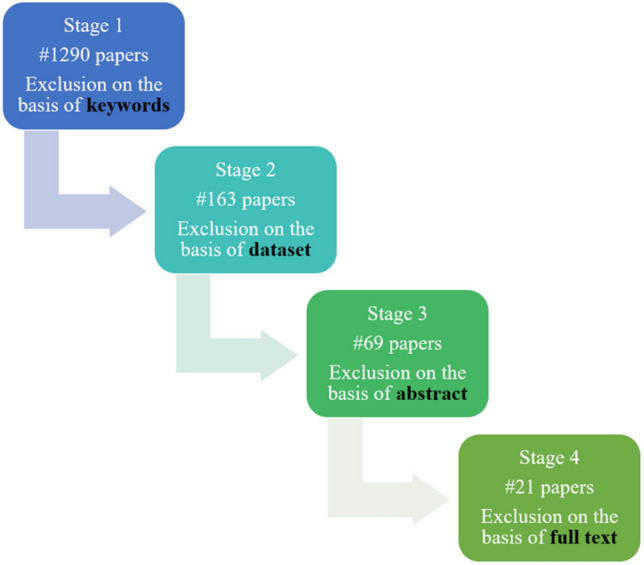
The literature review is focused mainly on studying the latest techniques proposed in the year 2020–2021 using the 2020 version of the BraTS dataset. The dataset is available at https://www.med.upenn.edu/cbica/brats2020/data.html. The criteria employed for inclusion or exlcusion of the research articles are described in Fig. 4. The Google scholar was used to find the required articles for this study. Initially, 1290 papers were obtained by conducting the search with keywords “brats”, “brain tumor”, “segmentation”, “survival” and “prediction”. Then, 163 papers were selected on the basis of 2020 version of the BraTS dataset. Further, 69 papers were selected on the basis of the abstract of the manuscripts. Lastly, 21 suitable papers finally met the inclusion criteria for this study.

Fig. 4.

Search criteria for selection of articles for the current study

The use of 3D MRI scans to segment gliomas aids in diagnosing and treating glioma patients. The BraTS challenge has been held yearly since 2012 as part of the International Conference on Medical Image Computing and Computer-Assisted Intervention (MICCAI) to assess current segmentation methods for pre-operative MRI-based BTS. The challenge makes medical data of GBM patients freely accessible for academic research purposes. This dataset contains a vast collection of pre-operative mMRI scans and clinical data with corresponding expert-derived ground-truth annotations across four MRI modalities [6, 22–25]. A considerable amount of research in BTS has been performed using the BraTS dataset [26–28]. The data are gathered from various sources, organisations, and scanners, including both LGGs and HGGs. The dataset contains training, validation, and testing data. For training data, segmentation ground-truth and patient’s survival information are provided. Validation and testing data, on the other hand, are devoid of segmentation indicators. Researchers can submit their results to the Centre for Biomedical Image Computing and Analytics (CBICA) Online Image Processing Portal to evaluate validation and test data performance.

The BraTS challenge 2020 consists of three tasks: segmentation of glioma brain tumour sub-regions, prediction of OS, and algorithmic uncertainty in tumour segmentation. The objective of the BTS task is to define the glioma and its internal components, including the WT, ET and TC. The SP task predicts the patient's survival time using the characteristics derived from MR imaging and clinical data. In recent years, the BraTS challenge has encouraged researchers to submit automated BTS and SP methods for evaluation and discussion using a publicly accessible mMRI dataset [6]. In the computer-aided diagnosis of gliomas, accurate BTS and SP are two crucial yet difficult objectives. Traditionally, these two activities were carried out independently, with little consideration given to their relationship. In order to extract robust quantitative imaging characteristics from a glioma image, it is necessary to accurately segment the three main sub-regions of the tumour image, viz. ET, TC and WT. Researchers think that these operations should be carried out in a cohesive framework to maximise the benefit.

Dataset

The objective of the BraTS 2020 challenge was to evaluate novel BTS and SP algorithms using pre-operative mMRI scans and clinical data. Various clinical techniques and scanners were used to collect data from a range of institutions [6, 22, 23]. In each patient's MRI scans, T1, T2, T1ce, and FLAIR (nifti files) are co-registered to the anatomical template of the T1 modality of the same patient. All patients in the training set are labelled (seg nifti file) for the three tumour tissues, i.e., ET, ED, and NCR/NET. All patient scans are skull-stripped and interpolated to $1\mathrm{mm}$ isotropic resolution. One to four evaluators segmented the images using the same labelling technique to prepare the ground-truth annotations. The annotations were validated by experienced neuroradiologists [24, 25]. The details are summarized in Table 1.

Table 1.

BraTS 2020 data for brain tumour segmentation

Data	Training	Validation	Testing	MRI voxel spacing	MRI dimensions
BraTS pre-operative MRI scans	369 (293 HGG, 76 LGG)	125	166	$1\times 1\times 1$	$240\times 240\times 155$

There were 236 patient data fields for patient survival statistics, including ID, age, OS (in days), and surgery status. GTR surgery was performed on 119 of the 236 data points, while the remainder underwent Subtotal Resection (STR) or Not Applicable (NA) operation. Out of 119 data with GTR status, one patient is alive; therefore, the datum used for survival training is 118. Based on this decreased number of observations, researchers created models to predict patient’s OS. The probability of survival days is divided into three categories: short term, mid-term, and long term. However, only patients with resection status GTR are considered for evaluation. The performance of proposed models can be assessed using validation and testing data. The details are highlighted in Table 2.

Table 2.

BraTS 2020 data for overall survival prediction

Data	Training	Validation	Testing
Clinical data (.csv data)	236 (119 GTR, 89 short, 60 mid and 87 long term survivors)	29	107

Brain tumour segmentation

Researchers solve the BTS task using clinically obtained training data by creating an algorithm and generating segmentation labels of the different glioma sub-regions. ET, TC, and WT are the three sub-regions that are being examined in BraTS 2020 BTS. As illustrated in Fig. 5, the provided segmentation labels have values of 1 for NCR and NET (red colour), 2 for ED (green colour), 4 for ET (yellow colour), and 0 for background (black colour). Researchers submit their segmentation labels for assessment as a single multi-label file in nifti (.nii.gz) format to CBICA Image Processing Portal.

Fig. 5.

MRI scans with segmentation labels in multiple views [6]

Survival prediction

The segmentation labels generated after performing BTS can be used to extract imaging/radiomic properties which can be used further to train machine learning (ML) and deep learning (DL) models to forecast the OS of GBM patients. It is not essential to limit the parameters to just volumetric features only. Researchers can even use intensity, histological, textural, spatial, glioma diffusion attributes and histogram-based features along with clinical features like patient’s age and resection status. The SP task requires a prediction of OS for patients with gross total resection (GTR). The prediction should be the number of days, and validation of the algorithm is dependent on the accuracy of categorization into three categories, viz. long survivors (greater than 15 months), short survivors (less than 10 months), and mid-survivors (within 10 and 15 months). The prediction results obtained by researchers are submitted as a Comma Separated Value (CSV) file, including the subject ids to CBICA's Image Processing Portal.

Generic workflow for brain tumour segmentation and survival prediction

Various end-to-end approaches for BTS and SP have been proposed in the literature. In some manner, all of these approaches assert their supremacy and usefulness above the others. In order to motivate researchers to present their automated BTS and OS prediction models, the BraTS challenge is organised yearly. It has been observed that the automated approaches accomplish the objectives of BTS and SP by following a similar set of steps. This section explains the generic workflow followed to predict the OS of patients, as shown in Fig. 6. SP models use pre-operative MRI scans and.csv data, including patient survival information.

Fig. 6.

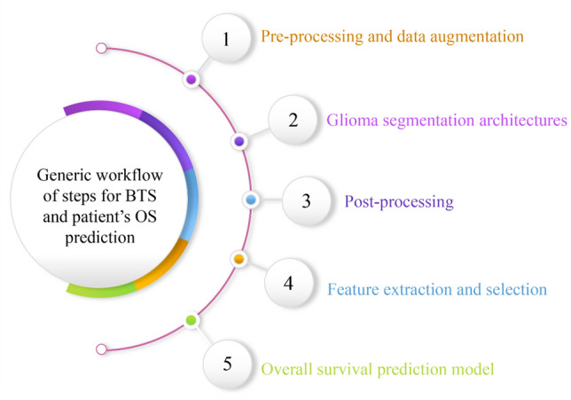
The generic workflow for brain tumour segmentation and overall survival prediction

Pre-processing and data augmentation

Deep convolutional neural networks (DCNNs) are data operating algorithms. These algorithms require vast data in order to come up with accurate conclusions. Pre-processing and data augmentation are essential since such big datasets are seldom available. In addition to standardising input data, pre-processing techniques can also enhance critical data inside the original input scan, such as cropping the area of interest when it includes redundant or misleading information.

Pre-processing

The BraTS 2020 challenge organisers provided pre-operative MRI scans and ground-truth annotations for the training set. To minimise variability in patient scans induced by imaging procedures, the coordinators supplied data that had been co-registered to the T1 anatomical template of individual patients, normalised to 1 mm isotropic resolution, then skull-stripped. Pre-processing improves network performance and training. As shown in Fig. 7, the authors [29–46] employed the following pre-processing methods to account for intensity inhomogeneity throughout the dataset.

1. Min–max normalization

Fig. 7.

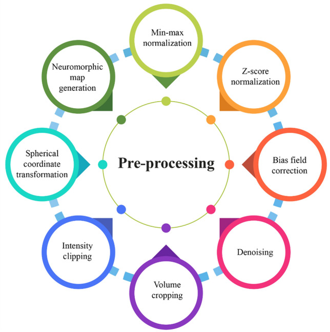
Types of pre-processing used in BraTS 2020 SP techniques

One of the most frequent methods for normalising data is min–max normalisation. ‘0’ and ‘1’ are the minimum and maximum values for each characteristic, respectively, and all other values are between 0 and 1.

$$\frac{\mathrm{value}-\mathrm{minimum}}{\mathrm{maximum}-\mathrm{minimum}}$$

value (image) = only the volume's brain area.

Although min–max normalisation ensures that all features have the same scale, it does not handle outliers well. Before feeding the MRIs as input for model training, González et al. [29], Parmar et al. [30], and Carmo et al. [31] normalised each MRI sequence in the range $\left[0,1\right]$.

• 2.z-score normalization

Researchers use z score intensity normalisation to minimise intensity variation within MRIs of different patients and variations among multiple modalities of the same patient. z score normalisation is a data normalisation method that eliminates the outlier problem. According to the formula given below, z score normalisation ensures intensity with a zero mean (mean) and a unit standard deviation (std) for each volume (considering only non-zero voxels):

$$\mathrm{image}=\frac{(\mathrm{value}(\mathrm{image})-\mathrm{mean}(\mathrm{image}))}{\mathrm{std}(\mathrm{image})}$$

value (image) = only the volume's brain area.

If the parameter ‘value’ is the same as the mean of all feature values, it is normalised to ‘0’; if it is less than the mean, it is a negative number; and if it is greater than the mean, it is a positive number. The original feature's standard deviation decides the magnitude of the negative and positive values. If the standard deviation of abnormal data is big, the normalised values will be closer to ‘0’. It deals with outliers but does not generate normalised data on the same scale. Researchers used z score normalization to set each MRI volume's mean and unit standard deviation before these volumes were fed into training models [29–42].

• 3.Bias field correction

In MRI scans, low-frequency bias field signals are very smooth that cause MRI corruption, especially when the MRI scanners are obsolete. There are differences in the magnetic field strength of MRI scans captured with different procedures and scanners across various institutions. Segmentation architectures, textural analysis, and classification techniques that rely on the grey-level values of image pixels will not provide satisfactory results. It is necessary to correct the bias field signals before submitting raw MRI data to automated algorithms. Agravat et al. [33], Patel et al. [35], and Soltaninejad et al. [40] used N4ITK Insight Toolkit [44] to reduce bias field in all available structural MRIs.

• 4.Denoising

MRI scans are often corrupted by Gaussian noise produced by the random thermal motion of electrical components and decreases image quality and reliability. Noise reduction can be achieved using a variety of noise filtering methods in order to improve image analysis. Agravat et al. [33] used denoising as a pre-processing step before training the segmentation architecture.

• 5.Volume cropping

Patel et al. [35] firmly cropped all MRI scans to eliminate empty voxels outside the brain area. The MRI data used for training and generating inference have been pre-truncated to a size of $160\times 192\times 128$ from the original image's centre point$.$ MRI volumes were similarly cropped by Akbar et al. [42] and González et al. [29] from the central point.

• 6.Intensity clipping

Pang et al. [43] reduced the amount of background region by using intensity trimming. Carmo et al. [31] also clipped MRI sequences within the interval $\left[-,5,,,5\right].$

• 7.Spherical coordinate transformation

Russo et al. [45] proposed spherical coordinate transformation as a pre-processing stage to improve segmentation results. Pre-training weights for future training stages were achievable due to the utilisation of spherical transformation in the first cascade pass. Extreme augmentation was also added via the spherical coordinate transformation. It was a practical step since it provides invariance for rotation and scaling. However, such invariance has disadvantages, mainly when dealing with WT segmentation; it introduces many false-positive areas. As a result, the authors employed a Cartesian model to filter away false-positive areas discovered via spherical pre-processing.

• 8.Neuromorphic map generation

Han et al. [46] used a neuromorphic inspired pre-processing technique for tumour segmentation. It followed the concept of attention-based learner combined with Convolutional Neural Network (CNN) to generate saliency maps which aided in better image analysis. This pre-processing technique mimicked the brain's visual cortex and enabled attention-based learning as a pre-determined method for predicting target object regions. During the BraTS 2019 challenge, the neuromorphic attention module demonstrated the effectiveness of training 3D objects with a 2D UNet constraint. The previous 2D UNet with neuromorphic attention module used three channels of incoming image data instead of the initial four channels [47]. Based on the generated saliency maps, this study analysed four-channel MRI data as three-channel input scans. The goal was to include neuromorphic characteristics into the input MRI data.

Data augmentation

Data augmentation, also known as artificial data generation, is a common approach used for improving the generalisation capabilities of Deep Neural Networks (DNNs). Data of good quality are hard to collect, and acquiring new examples is also very time-consuming and expensive. Medical image analysis, especially tumour delineation, is affected by this problem [48]. Several data augmentation techniques were used by researchers to increase the number of training samples which included random axis mirror flips [29, 30, 33–38, 49], intensity scaling and intensity shifting [31, 34, 37], isotropic scaling, per-channel gamma corrections [35], rotations [35–37, 43, 49], random scaling [38], elastic transformations, and zoom-in and zoom-out [49]. There are many ways of augmenting MRI scans, as illustrated in Fig. 8.

Fig. 8.

Different forms of data augmentation [48, 50]

Glioma segmentation architectures

ML approaches, particularly DL architectures, have been applied recently in the medical domain to improve diagnostic and treatment procedures by building automated systems to categorise patients, regression-based predictions, and semantic segmentation applications [51]. However, due to data availability constraints, automation in medical applications is a big challenge. An unbalanced dataset is a common problem in medical imaging. For example, the cancer area is small relative to a healthy brain and MRI scan background. Creating a good DL structure, in general, is challenging, but it is now essential to automatically process data of the vast number of patients. Significantly, a deep structure can generate a wide range of features without the researchers' input. ML models are suitable for tiny datasets, but researchers need significant characteristics to train such models. ML/DL limitations have been addressed in many ways. Standard techniques for overcoming the imbalanced data problem in segmentation problems include the Weighted cross-entropy loss (WCEL) function, the generalized dice loss (GDL) function, and balanced patch selection [52]. Pre-processing techniques, such as volume cropping, data denoising and augmentation, have also led to improving the performance.

The accuracy of automated diagnostic systems has been improved by using several different models [53–57]. 3D MRI with DNNs is now widely used to diagnose brain tumours because of their valuable and precise performance. Artificial neural networks (ANNs), such as fully convolutional neural networks (FCNNs) and their ensembles, contribute to the medical field by automatically segmenting the tumour's sub-regions. Accurate BTS algorithms are needed more when the machine observes volumetric MRI scans in three dimensions rather than the actual two-dimensional (2D) perspective of a human interpretation. Even though mMRI provides complete information, it is still difficult to differentiate all sub-regions due to false image features. DL-based approaches often outperform standard ML methods for image semantic segmentation [23].

In their work [58], the authors covered the fundamental, generative, and discriminative approaches for BTS. DNN has recently gained popularity for the segmentation of radiological scans. DeepMedic [27], UNet [59], V-Net [60], SegNet [61], ResNet [62], and DenseNet [63] are the examples of CNN that generate semantic segmentation maps. UNet is generally acknowledged as a standard backbone architecture to perform semantic segmentation in medical imaging. UNet is an encoder–decoder architecture that reduces feature maps to half on the encoder path and doubles feature maps on the decoder path. The skip connections between UNet's parallel stages aid in feature reconstruction.

Due to the volumetric structure of MRIs, organs are often scanned like 3D entities and subsequently segmented using 3D CNN-based architectures. Myronenko et al. [56] (BraTS 2018 winner) proposed a variational autoencoder-based 3D encoder–decoder architecture for BTS. Isenee et al. [64] (second in BraTS 2018 challenge) utilised a modified version of the basic UNet [59] using diligent training and data augmentation throughout the model training and testing phase. The performance improvement was observed when Leaky Rectifier Linear Unit (ReLU) was utilised instead of the ReLU activation function. The BraTS 2019 winner, Jiang et al. [55], employed a two-stage cascaded UNet architecture to segment brain tumours. Different tricks for 3D BTS, such as sampling of patient’s input data, random patch size-based training, semi-supervised learning, architecture depth, learning warm-up, ensembling, and multiproblem learning, were used.

Model training and hyperparameter tuning are essential issues related to the high resource consumption by these models. 2D Neural Networks (NNs) have fewer parameters than 3D models and can be trained quickly, which allows for better hyperparameter tuning. Due to the absence of depth information, the 2D UNet performs poorly in 3D segmentation. As a result of class imbalance and increasing computing expenses, 3D UNet-based models often face many difficulties. Many recent studies have utilised ensemble models that average the output probabilities of separate models to enhance generalisation power and segmentation performance by providing uncertainty estimate for each voxel in the vision [55, 56, 64–67]. Due to different weights and hyperparameters used for model optimisation, individually trained models vary in one way or the other. As a result, ensembles have certain disadvantages like training time, memory constraints, and increased model complexity. New versions of the UNet were developed by Isensee et al. [54, 64] to show that a well-trained UNet can outperform complex ensemble approaches. Many later-year submissions that attempted to utilise the modified 3D UNets or ensembles of 3D UNets [55, 56, 68] seem to be inspired by Isensee's work. The glioma segmentation architectures used in BraTS 2020 SP task to segment tumour sub-regions are classified in Fig. 9.

Fig. 9.

Different types of networks used for glioma segmentation

Single networks

Using a three-layer deep 3D UNet encoder–decoder framework, Agravat et al. [33] presented a tumour segmentation architecture with deep connections to increase network depth. It enabled the gradient to flow straight to the previous layers, allowing the classification layer to watch the preceding levels closely. The layers' extensive connections further enhanced the difficulty in identifying patterns. An unbalanced dataset caused problems with BTS with a higher proportion of non-tumourous slices than tumourous slices, which reduced network accuracy. The 3D patch-based input ensured that the network did not overlearn the background voxels. The network was trained using a mix of dice loss and focal loss functions to enhance its performance to address this class imbalance. A smaller subcomponent size (NCR and ET) contributed to the failure of the network, especially in LGG cases.

Using an accumulated encoder (AE), Chato et al. [69] developed a modified 3D UNet consisting of three layers of encoder/decoder modules with concatenation links. AE included ReLU, accumulated block (AB), and max-pooling. To enhance the quality of low-level features, the AB developed two feature maps depending on element-wise addition. After a last max-pooling layer, two branches of convolutions generated these feature maps. After clipping the training patch, channel normalization (CN) [70] was applied to prevent overfitting and solve the class imbalance problem. In order to trigger the training procedure with network convergence and performance improvement, the mini-batch method was employed. After two convolutional layers, each encoder unit had batch normalization (BN) [71], a ReLU, and a max-pooling layer.

Anand et al. [32] suggested 3D FCNN with encoding and decoding pathways. Dense blocks and Transition Down blocks were used in the encoding route. A limited number of output feature maps were chosen for each convolutional layer to avoid the parameter explosion. The spatial dimension of the feature maps was decreased using the transition down blocks in the network. Dense blocks and Transition Up blocks make up the network's decoding or up-sampling route. The reversed convolution layers were used in the Transition Up blocks to move sample feature maps up in the hierarchy. The features from the encoding portion were combined with the upsampled features as input for the dense blocks in the decoding phase. With complicated cases, the suggested network did not perform well. The trained network was fine-tuned, and hard mining was conducted on tough instances [72]. With the help of DSC, a threshold-based selection of complicated instances was made.

Parmar et al. [30] showed that an increase in batch size might lead to smaller patches with less contextual information. Contrarily, a bigger patch size may provide more contextual information, resulting in smaller batch size, raising the stochastic gradient variance, and reducing the amount of optimization achieved. Batch pools with varying patch sizes were created. The model could learn global information from the most prominent patch and relevant texture from the minor patch with the same parameters by employing various cropping and padding stages between the convolution layers. Patching would also enable a less powerful Graphical Processing Unit (GPU) to handle the big image. The down block of the UNet framework [54] lowered patch size and increased channel length. Overfitting was eliminated by using the down block, which transmitted data from front to end. The position information was reconstructed using the down block outputs, which were then combined in the up block. Based on the probabilistic matrix, the patch size and number of channels were determined. Setting appropriate threshold values for each class helped to accomplish this goal.

Glioma segmentation was solved by Pang et al. [43] by using a 2D encoder-decoder arrangement. The encoder portion utilised five Feature Mining Units (FMUs) and four downsample modules to encode the input data. With the use of this structure, the input data may be cleaned of the noise while retaining the crucial features that made segmentation possible. Each of the convolution kernels utilised in the FMU interacted via skip connections; the characteristic channel information collected from these processes was spliced together [73–75]. All convolution operations were combined with BN operations [71] and ReLU activation functions. The decoder's FMU had the same structure as the encoder's. At the same time, the output datum of each FMU in the decoder was up-sampled to the original size of the image to maintain fundamental patterns. As a result, incorrect information was eliminated, and only appropriate data persisted [76, 77].

Suter et al. [78] used the usual ground-truth labelling for cerebrospinal fluid (CSF), WM and grey matter (GM) acquired using FSL software [79] to train a nnUNet-framework [80] for locating healthy areas. All images were subjected to an MRI modality-specific piece-wise linear intensity transformation based on these healthy tissue labelling to complement the healthy tissue intensity and map to a set intensity range for consistent grey-value binning. Only the WM and GM labelling were utilised, and CSF segmentation was frequently compromised by insufficient skull-stripping. The N4 method [44] was used to correct the bias field in all of the images.

To extract the local characteristics of the tumour, Zhao et al. [38] developed a segmentation then prediction (STP) architecture trained on patches. A global branch retrieved the WT's global characteristics to forecast survival days. An encoder and a decoder were used in the segmentation module. Eight convolutional blocks and three downsampling layers comprised the encoder part. There was a downsampling layer between every two convolutional blocks. Because of the limited GPU memory, the group normalization (GN) [81] was substituted with the IN. An output layer followed three pairs of upsampling stages and convolutional blocks in the segmentation decoder. Convolutions were used in an upsampling layer, followed by trilinear interpolation and skip connections between the encoder-decoder paths. The number of channels in each convolutional block was decreased to half of the channels in the preceding block. The output layer included convolutional kernels and three channels to generate the ET, WT, and TC segmentation masks.

Patel et al. [35] hypothesised that networks using conventional convolutions were less capable of producing correct segmentation labels for glioma sub-regions. As a result, the authors suggested inserting modified selective kernel (SK) blocks [82] into the recommended UNet. An attention mechanism allowed the network to automatically change its receptive field to accommodate spatial information collected at various scales. Due to the limitations of GPU memory, the suggested framework learned both anatomical context and complex representations. Downsampling and upsampling of feature maps were achieved via max-pooling with trilinear interpolation, which further helped in decreasing the network's memory footprint. Deep supervision [67, 83] was used to promote quicker network convergence. The proposed SK blocks may be broken down into three operations: (1) split, (2) channel selection, and (3) spatial attention. A channel attention technique was used to enable the network to alter the receptive field of the SK block adaptively. A primary spatial attention mechanism, comparable to the convolutional block attention module [84], was used to make the network concentrate more on prominent image regions. The channel datum was aggregated using the max and average pooling methods across the channel dimension.

Dai et al. [36] used the UNet attention framework (UNet-AT) for BTS, which made use of attention-gated blocks' capacity to focus more on semantic information to improve segmentation performance. Further, there was no need to increase effort for fine-tuning the model parameters and pre-process the data. IN was selected at random for the UNet-AT. The activation function is Leaky-ReLU with a leakiness of 0.01.

McKinley et al. [37] used DeepSCAN, a 3D-to-2D FCNN that performed well in the 2019 BraTS challenge [66] and was trained using uncertainty-aware loss. The instances were classified based on confidently segmented core or a poorly segmented or missing core. It was assumed that every tumour had a core. Thus, the criterion for classifying core tissue was lowered when the core, as delineated by the classifier, was poorly defined or absent. The network started with 3D convolutions to compress a non-isotropic 3D patch to 2D. In the bottleneck, a shallow encoder/decoder system utilised densely linked dilated convolutions. This architecture was extremely similar to the authors' BraTS 2018 proposal. The main changes were that the authors utilised IN rather than BN and included a basic local attention block across dilated dense blocks.

Cascaded networks

Using the DeepLabv3+ [85, 86] model, Miron et al. [34] developed a version of a two-stage cascaded asymmetric UNet in which decoders kept track of the segmentation region contour to add more regularisation. Large dimensions were used to protect global information. Due to memory constraints, a two-branch decoder with interpolation and deconvolution was employed on the first level of the cascaded model. Model inputs were initial volumes concatenated along with segmentation maps produced from the first step. Two different convolutions were applied to the segmentation and outline of the segmentation region as a regularisation step. Shorter decoders were able to retain more information throughout the upsampling process. When needed, residual additive connectors were added. In order to extract features at different resolutions, the encoder was changed by adding atrous convolutions having varying dilation rates. A Spatial Pooling unit was introduced in the encoder to make use of the dilated convolutions. After combining the five feature maps, the decoder received them as a single data stream. There were two output tuples at this point: one acquired via upsampling and the other through transposed convolutions.

In contrast to conventional Cartesian space imagery and volumes, Russo et al. [45] presented a new technique for feeding DCNN with spherical dimension converted input data to improve feature learning. The DCNN used as a baseline for the proposed approach was developed from the work of Myronenko [56], built on a variational auto-encoder (VAE) UNet with modified input shape and loss function depending on the kind of transformation employed in the pre-processing phase. The VAE consisted of a UNet comprising two decoder divisions: a segmentation decoding branch used to get the ultimate segmentation and an extra decoder used to regularise the shared encoder. For COVID-19 severity evaluation and progression prediction [87], the lesion encoder (LE) architecture was suggested. The original LE used the UNet structure [59], which included an encoder and decoder inspired by the EfficientNet [88]. The decoder translated the lesion feature maps to the input MRI size and produced the segmentation maps while the encoder learnt and recorded the lesion features in the input images.

Tumour- EfficientDet (T-EDet), a variation of EfficientNet [88], was suggested by Carmo et al. [31]. Using a pre-trained EfficientNet [88] with D4 variant, the calculations of backbone weights and features were the starting point for EfficientDet. Because the initial network was developed with a 3-channel input, a significant issue emerged with varying input channels. The 4-channel (4 modalities) input was converted into a 3-channel input using an adaptation convolution. The Bi-directional Feature Pyramid Network (BiFPN) altered the characteristics obtained from the pre-trained EfficientNet to get its initial features. A transposed convolution accompanied by BN and the same swish activation [89] was employed to adapt this representation to the size of the input MRI data. This new representation was given to the segmentation architecture. It comprised three blocks of depth-wise convolutions [90], batch norm, and swish, coupled with a final convolution to reduce the number of classes. In isolation and then as the backbone of the planned multiproblem experiment, the UNet 3D architecture based on the work of Carmo et al. [91] was utilised. In terms of training technique, several hyperparameters comparable to Isensee's work [54] were used. The primary experiment included the end-to-end refining of segmentations generated by a solid pre-trained UNet 3D backbone model, as well as the inclusion of an attention-based SP branch.

Self-ensemble network

Pei et al. [39] presented a technique based on 3D reUNet DL. The reUNet was made up of a standard residual ResUNet and a self-ensemble model. The problem of gradient vanishing stopped with the use of the self-ensemble model and the ResUNet model. For OS prediction, the tumour segmentation probabilities derived from 3D Self-ensemble ResUNet (srUNet) were utilised. Even though DL-based techniques performed well in semantic segmentation, a large number of training samples were needed.

Parallel network

Soltaninejad et al. [40] presented a segmentation method that consisted of two major branches with varying degrees of resolution. Based on the technique described in Newell et al. [92], the native resolution branch was an encoder-decoder architecture with residual blocks. In the last layer, the activation function was changed with a sigmoid function. The native branch dealt with better resolution small-sized MRI patches. For segmentation, another branch with a broader view but a poorer resolution was added. In order to match features from the larger receptive field with the native branch, these features were trimmed. As a final step, the characteristics from both branches were combined and presented to the final layer for segmentation. In order to create the delineation heatmaps from the features, two convolution layers were utilised for each path. In order to train the network, several loss functions were employed, such that each branch learned relevant characteristics together with the final layer. The output was sent through a Sigmoid function which used stochastic gradient descent to learn the network's topology to train the network. For each class, a separate model was trained against all other labels to identify patterns.

Ensemble network

When it comes to the BTS task, González et al. [29] presented an ensemble of seven models with 3D and 2D input methods, all based on asymmetric UNet (AUNet). According to the 2.5D model, each modality's low-level characteristics were extracted separately using a multi-input approach. Multi-view 2.5D Inception block was designed to combine features from various perspectives of a 3D visual and accumulate multi-scale features into a single 3D image. Five layers were used in the enhanced 3D UNet to extract additional semantic information, with the encoding route having twice the number of convolutional blocks as the decoding path. There were four 2.5D Multi-View Inception blocks and a modified 3D UNet architecture that included residual blocks, instance normalization (IN) [93], transpose convolutions for performing upsampling, and additive skip connections within encoding and decoding paths in the multi-input module.

Ali et al. [41] suggested a combination of 2D and 3D approaches to maximise their advantages. The authors also showed that if hyperparameter tuning was done effectively, 2D models might attain comparable or even better performance than 3D models. Several axial, sagittal, and coronal views were used to train the model to compensate for the absence of depth information in 2D models. A combination of 2D and lightweight 3D models was used to train the ensemble model introduced by Asra et al. [94] to extract both 2D and 3D benefits. The 3D dilated multi-fiber network (DMFNet) [53] model was selected because fewer parameters could be learnt more rapidly than other 3D complicated models. MultiFiber (MF) and dilated convolutions were used with group convolutions to decrease parameters and preserve prediction precision. The information was sent using a multiplexer between the fibres by combining two convolutions with the four-channel input. The spatial information of brain tumours was then captured using dilated convolutions. Convolutions were performed with multiple dilation rates to check how many pixels were missed throughout the process. An ensemble of these two models was constructed in order to make use of both.

Zhang et al. [95] focused on utilising the brain parcellation-based knowledge, coarse-to-fine approach, and ensembling to enhance UNet segmentation performance. Four UNets were trained independently to perform BTS. UNet1 investigated how distinct tumour areas were more apparent in various MRI modalities. UNet2 focused on developing a brain parcellation prototype using a T1 MRI as input. Brain parcellations plus mMRI images were used to train UNet3. Utilizing cropped MRI as well as brain parcellations as input, UNet4 resulted in coarse-to-fine segmentation. The final output was achieved via a majority vote of both coarse and fine segmentation. Table 3 summarises the specifics of segmentation architecture used to segment tumour sub-regions before performing feature extraction.

Table 3.

Summary of segmentation architectures for BraTS 2020 SP problem

Authors	A	B	C	D	E	F	G	H
González et al. [29]	Ensemble	2.5D, 3D	AUNet	5	Inception block (2.5D), residual block (3D)	IN	Multi-input strategy	Five-fold cross-validation
Agravat et al. [33]	Single	3D	Encoder-Decoder FCNN	3	Dense module	BN	Deep supervision	–
Miron et al. [34]	Cascaded	3D	Two-stage cascaded asymmetrical UNet	3	Residual additive connections, spatial pooling module, Atrous convolutions with dilations	GN	Regularization by contouring	–
Chato et al. [69]	Single	3D	UNet AE	3	Accumulated block	CN, BN	Information fusion strategy	–
Anand et al. [32]	Single	3D	FCNN	3	Dense blocks, transition up/down blocks	–	Hard mining on complex cases	Stratified sampling
Parmar et al. [30]	Single	3D	UNet	5	Downblock/Upblock	IN	Patch selection strategies	Stratified sampling
Soltaninejad et al. [40]	Parallel	3D	Encoder-Decoder	2	Residual block	–	Multi-resolution method	–
Pang et al. [43]	Single	2D	Encoder-Decoder	4	Residual units	BN	More abundant features	–
Ali et al. [41]	Ensemble	2D, 3D	2D UNet and 3D DMFnet	3	Group convolution with MF, dilated convolutions	–	Utilized 2D and 3D benefits	–
Russo et al. [45]	Cascaded	3D	DCNN	3	ResNet block in variational autoencoder	–	Spherical coordinate transformed input adds extreme augmentation, variational autoencoder-based UNet	–
Akbar et al. [42]	Parallel	2D	MobileNetV1/V2	3	Removed classification part, additional layers to produce the ratio of tumour sub-regions	BN	Focused on DL-based feature extraction rather than segmentation	Stratified sampling, fivefold cross-validation
Marti Asenjo et al. [49]	Single	3D	EffUNet	5	EfficientNet block in encoder	–	Deep supervision	–
Carmo et al. [31]	Cascaded	3D	T-EDet	5	D4 variation of EfficientNet, bi-directional feature pyramid network (BiFPN), multiATTUNet	BN, GN	Modification of 2D semantic segmentation EfficientNet model, MultiATTUNet architecture	–
Han et al. [46]	Single	2D	UNet	4	Neuromorphic attention-based learner	BN	Neuromorphic saliency map	–
Pei et al. [39]	Self-ensemble	3D	srUNet	4	Regular ResUNet and srUNet model	–	Self-ensemble avoids gradient disappearance and regularises training	–
Suter et al. [78]	Single	3D	nnUNet-framework	5	Piece-wise linear intensity transform, grey-level binning	IN	Identified healthy region labels for CSF, WM, GM	Five-fold cross-validation
Zhao et al. [38]	Single	3D	Encoder–decoder	4	Residual connection	IN	STP with local and global branch	Five-fold cross-validation, self-training
Patel et al. [35]	Single	3D	UNet	5	Selective kernel block with attention mechanism, residual bottleneck block	GN	The network adjusts its receptive field via an attention mechanism, deep supervision	–
Dai et al. [36]	Single	3D	UNet-AT	5	Attention-gated block	IN	Self-training model again with the training set and previously generated pseudo annotations for the validation set	–
McKinley et al. [37]	Single	3D-to-2D	DeepSCAN	–	Dilated dense block with attention	IN	Separate cases based on confidently segmented/ vaguely segmented/ missing core	–
Zhang et al. [95]	Ensemble	3D	UNet	4	Brain parcellation model using T1 MRI	–	Use of brain parcellation, coarse-to-fine strategy	–

A Network type, B Input dimension, C Segmentation backbone, D Depth/levels/layers, E Modifications, F Normalization, G Uniqueness, H Sampling

Post-processing

Several post-processing techniques for eliminating false positives and improving segmentation results have been suggested. Traditional post-processing techniques, like threshold- or region-growing methods, focus on isolated regions or pixels by utilising manually defined thresholds. Recently, post-processing techniques such as Connected Component Analysis (CCA), Conditional Random Fields (CRF), and Gaussian Markov Random Fields (MRF) have been utilised to infer pixel pairings given previous information such as pixel intensity distributions and geographic distance. Recently, the researchers coupled CRF to NN models in an end-to-end learning manner for image segmentation issues [96]. The post-processing shown in Fig. 10 increased the DSC and HD95 of the ET, WT, and TC classes considerably.

Fig. 10.

Post-processing techniques used by SP techniques submitted in BraTS 2020 challenge

Connected component analysis

CCA cluster voxels depending on connectivity and voxel intensity levels are comparable. The highly tiny linked components are removed from the result since they are false positives due to misleading segmentation findings. Agravat et al. [33] chose CCA to eliminate the tumour, which had a volume of less than one thousand voxels. To post-process the segmented labels, Anand et al. [32] utilised class-wise 3D CCA. Marti et al. [49] defined the primary tumour volume as the most considerable linked (solid) volume. Over the training dataset, the distance from each smaller area (secondary tumour volumes) that was not linked to the primary tumour was computed. After tumour segmentation, the secondary volumes situated at a distance more significant than the average range plus 1.5 times the normal deviation were deemed false-positive and; were therefore eliminated and categorised as background. Patel et al. [35] used CCA to minimise the frequency of false positives in any class with fewer than ten voxels. Zhao et al. [38] used CCA to enhance segmentation performance as well. Dai et al. [36] eliminated a tiny isolated WT/ET (just under ten voxels) out from prediction, modifying the TC size to match the size of the ET.

Conditional random field

The algorithm assumes the voxel category based on characteristics linked to a specific voxel, independent of the voxel's connection to other adjacent voxels. CRF analyses this connection and creates a graphical model to handle prediction dependencies. CRF was employed by Anand et al. [32] to smoothen the segmentation maps.

Morphological operations

Morphological operations were used to modify voxel values depending on their neighbourhood, taking into account the size and form of the voxel. After screening the spherical segmentation using the Cartesian filter, Russo et al. [45] utilised post-processing to improve ET segmentation. The scientists discovered that isolated voxels were responsible for numerous erroneous positive ET segmentations. The scientists used a binary opening operation to separate thin branches across ET sites before filtering out those with less than 30 voxels. Whenever the ET segmentation remained after these filters, the original was recovered and utilised as the final one. Alternatively, the ET partition was deleted, implying that there was no ET in the current volume.

Relabelling the output label

González et al.[29] established a threshold value that represents the smallest size of the ET area. When the overall amount of predicted ET voxels was less than the threshold, the label of all voxels in the ET area was substituted for one of the NCR regions. In the validation dataset, the threshold value was calculated to obtain maximum performance in this region. If the segmentation model did not identify a TC, the authors concluded that the identified WT area matched the TC and relabeled it as TC. ET was produced in the vicinity of the NCR, according to Agravat et al. [33]. Furthermore, in HGG, its size cannot be minimised. Because of its tiny size, ET was changed to NCR. Three hundred was the experimentally determined threshold for relabelling. As a post-processing step, Carmo et al. [31] used a particular threshold in ET segmentations, where segmented regions with less than 300 voxels were utterly wiped out. It was done to prevent false-positive predictions of the ET region, which may cause DSC to be zero in individuals without ET. According to Patel et al. [35], most LGG patients have no ET portion, and the inclusion of even a single misdiagnosed ET voxel in estimated label maps leads to a DSC of 0. To mitigate the severity of the penalty, the authors substituted all ET voxels by TC if the number of anticipated voxels was less than 50. Zhao et al. [38] discovered that if the segmented ET was less than 350 voxels, the authors suspected no ET in LGG instances and removed those identified voxels from its segmentation result.

Feature extraction and selection

Radiomics is studied to investigate the relationship between medical imaging aspects and underlying biological properties. It is a technique of extracting efficient quantitative characteristics from radiographic scans and developing prediction architectures that link image attributes to clinical outcomes. The fundamental concept behind radiomics is that intra-tumour imaging heterogeneity can be retrieved from the MRI scans. The tumourous areas estimated from the patient's MRI volume were then utilised to predict OS time.

González et al. [29] used four MRI modalities to derive radiomic characteristics from the whole brain and five sub-regions. WT, TC, ED, NCR, and ET are the feature extraction sub-regions. The Python library PyRadiomics [97] was used to extract all 2568 handcrafted features. The recursive feature elimination (RFE) method was employed to reduce features to prevent overfitting. Radiomics was also used to estimate two additional characteristics: the relative invasiveness coefficient (RIC) and relative necrosis coefficient (RNC). Agravat et al. [33] collected the patient's age, statistical data, and NCR shape for the SP model.

Miron et al. [34] retrieved radiomic characteristics from segmentation labels, which primarily defined the area of interest's 3D shape, size, and centre of mass. Each tumour sub-regions ratio to the total brain size and the WT were included. A new binary characteristic called ‘High Risk' was set, if the tumour was in the lobe with a higher risk probability or in the left hemisphere. A greater risk was assessed if the centre of mass was located within 128–150 slides (sagittal plane), 60–150 slides (coronal plane), or 0–41 slides (transversal plane).

Chato et al. [69] utilised a feature-level and decision-level information fusion approach for creating the OS prediction model. The intersection of two brain midplanes splits a brain volume into four or eight tiny sub-volumes to retrieve volumetric characteristics. Five volumetric features indicating the volume of a brain region/WT/ET/NCR-NET/ED were gathered from each tiny volume, plus the volume of the whole brain and the WT. The centroid, volume, diameter, orientation, principal axis length, surface area extent, and solidity of the tumour site were among the twenty-eight shape and location characteristics. Only GTR resection status was considered for evaluation. There were 119 samples with GTR resection status out of 236 samples in the BraTS 2020 training dataset. A dataset of 119 samples was insufficient to build a reliable OS prediction model. Thus, resection status was utilised as an additional non-imaging characteristic (i.e., GTR as ‘1’, STR or NA as ‘0’). The patient's age was utilised as another non-imaging characteristic since it was one of the variables considered by physicians to select an appropriate treatment strategy for glioma patients.

Anand et al. [32] extracted radiomic features such as mean, median, and entropy, as well as second-order features such as Gray Level Co-Occurrence Matrix (GLCM), Gray Level Run Length Matrix (GLRLM), Gray Level Dependence Matrix (GLDM), Gray Level Size Zone Matrix (GLSZM), and Neighboring Gray Tone Difference Matrix (NGTDM). A total of 1022 distinct characteristics were retrieved using a different mix of segmentation maps. Each characteristic's significant value was given using a forest of trees [98, 99].

Volume and shape characteristics were derived from the whole brain and tumour substructures by Parmar et al. [30]. The 2D/3D diameter, major axis, minor axis, elongation, spherical index, whole brain’s flatness, and tumour sub-regions were retrieved to identify interrelationships as shape characteristics. For matching segmentation labels, a clinical characteristic (age) was assigned.

For SP, Soltaninejad et al. [40] used statistical characteristics of already segmented tumour areas from the previous segmentation step. The volume sizes of the WT, TC, and ET that were normalised w.r.t. the total brain volume were considered. The mean intensities for each tumour tissue type, i.e., the WT, TC, and ET, was another set of characteristics. As a result, eight characteristics were utilised for OS prediction.

Pang et al. [43] extracted characteristics from MRI data by masking the ED, ET, and NCR-NET regions. The particular feature selection procedures included Cox univariate analysis, Cox multivariate analysis, and the ph hypothesis test. Minor axis length, sphericity derived from the segmentation result using the ED mask, and busyness extracted from the segmentation result using the ET area mask were among the selected attributes. In addition, the patient’s age was included in the final feature set. According to a bivariate study, the patient's age and survival time were substantially linked at 0.01. The Pearson correlation value was -0.353, which suggested that the patient's age can affect OS.

To estimate the OS time, Ali et al. [41] collected radiomic and image-based characteristics. The image-based characteristics were volume, surface area and ratios, and the WT and ET centre positions. The Laplacian of Gaussian (LoG) filters was used to extract radiomic characteristics. The input image's texture and intensity-based characteristics were retrieved and filtered using LoG filters with sigma values 1, 2, and 3. Fourteen shape-based characteristics (tumour volume, diameter, surface area), first-order features, and GLCM features were recovered from segmented tumours. The characteristics for the tumourous areas ET, ED, TC, and WT were extracted. Because of tumour overlapping, some features were common. The top-performing features were chosen using Random Forest (RF) Recursive Feature Elimination. The patients' age was included in the feature vector since it provided crucial information about their survival.

Individual lesion encoders were utilised by Russo et al. [45] to extract the latent variables of the input MRI scans, which were further used as input parameters to predict patient OS. A high-dimensional feature vector (d = 256) was generated for each MRI scan. Principal Component Analysis (PCA) regulated the feature dimensionality by selecting various principal components for subsequent analysis since the high-dimensional feature space tended to overfit. The age distribution seems normal; however, the OS distribution appears skewed, with most instances having an OS of fewer than 400 days. The tailed distribution of the OS values was modelled using a Tweedie distribution.

Akbar et al. [42] suggested modifying MobileNet V1 and MobileNet V2 as interchangeable feature extractors. The predictive architecture was fed with extracted features and patients’ age data. The MobileNet V1 design was changed by eliminating a portion of the categorization and linking it to many additional layers, resulting in three characteristics (the ratio of NEC, ED, and ET area to the overall area of the tumour). MobileNet V1 received a two-dimensional image with three channels that were a multiple of 32 in size. In contrast, the accessible dataset consisted of four cropped 3D images from the image's centre. T1ce, T2, and FLAIR images were utilised to modify. Axially sliced 3D MRI scans were obtained, yielding 128 2D image data of $160\times 192$. The three images were stacked as three channels, and the 128 slices were converted into batch numbers for a single epoch. A dropout with a factor of 0.1 was employed to avoid overfitting [100]. Similar changes were made to the MobileNet V2 design, except that the output feature was used instead of the categorization layer. The same approach was used to input 3D MRI images to this architecture, as in the MobileNet V1 design. MobileNet V2-based modified network was selected based on the test findings.

Marti Asenjo et al. [49] created three distinct datasets for each patient's 2D anatomical plane, i.e. axial, sagittal, and coronal. The identification of low-level characteristics was enhanced by using a pre-trained EfficientNet network [88] based on ImageNet [101] as the UNet encoder Efficient UNet (EffUNet). This idea was to expand the number of layers and channels. The 3-channel decoder input layer was pre-trained on ImageNet, and further upgraded to a 4-channel configuration to accommodate all MRI modalities for each patient. The fourth layer was seeded with random weights drawn from a Gaussian distribution. The Laplacian and tumour gradient were vital in glioma tumour growth models [102, 103]. For all MRI sequences and the segmentation matrix, the Laplacian and the vector module of the 3D gradient were derived. Transformations were performed using MRI images (pixel values) and segmentation masks for a particular area, resulting in a binary matrix with ‘1’ within and ‘0’ outside the specified region. A complete tumour contains the whole of all three groups. NCR/NET volume, Gross Tumour Volume (GTV), and WT were also included in three ring-shaped structures. Following extraction, dimensionality reduction was required to select those characteristics with a higher connection to patient survival. Geometrical, statistical, locational, textural, and other characteristics were retrieved. Three variables (GTR, STR, and NA) were added as categorical and binary characteristics. Three distinct feature selection techniques were used: fscchi2 (ranking for classification using chi-square tests), fscmrmr (ranking for classification using Minimum Redundancy Maximum Relevance (MRMR) algorithm) and fsrftest (ranking for regression using F-tests). Each algorithm was then assigned the significance of each feature.

Han et al. [46] developed the neuromorphic saliency map to improve image analysis. An attention and saliency map was created to enhance tumour segmentation by simulating the visual brain and applying neuromorphic pre-processing. Several orientation-selective characteristics were used to build the neuromorphic NN. The orientation selectivity inspired by the visual cortex's "simple cell" enabled the resilience of abstract feature extraction [104]. The authors were able to generate a saliency map using the down-up resizing network. The saliency map proved successful at either eliminating noise or attracting attention. A new abstract image was created using UNet and a neuromorphic NN mixed network for BraTS 2019 [47]. It demonstrates the possibility of using a neuromorphic NN for image pre-processing or image post-processing.

Pei et al. [39] retrieved shape characteristics from segmentations produced and included non-radiomic variables like age. In the training phase, features were chosen based on their significance using an RF classifier based on survival risk. Data were randomly divided as training and validation in an 8:2 ratio in the training phase to determine the feature significance. The number of NC, ED, ET, shape elongation, flatness, most petite axis length, and surface area were among the 34 characteristics retrieved.

Suter et al. [78] retrieved features using the PyRadiomics library [105] for all four MRI modalities and the two segmentation labels WM and GM. The LoG filtered, intensity-based features were extracted for the original wavelet image. For tumour location characteristics, the images were registered using the MNI152 atlas [106]. Because the tumour's mass impact often altered the ventricles' location and shape, the authors used the Symmetric Normalization (SyN) [107] to reshape the afflicted regions appropriately. In the first stage, the authors eliminated any characteristics having a concordance index (cindex) less than 0.55. For all feature pairings having a correlation coefficient of 0.95 or above, the authors progressively eliminated the feature with the lowest c-index. The use of two priors was investigated. When the sequence prior was used, the characteristics were restricted to the T1ce and FLAIR MRI images. Features having an Intraclass Correlation Coefficient (ICC) (2, 1) of 0.85 or above were evaluated for robustness prior. These priors were evaluated both individually and together. Many ML techniques need or benefit from regularly distributed target variables. All sixteen feature selection and eleven ML technique combinations were examined. ReliefF (RELF), Fischer score (FSCR), chi-square score (CHSQ), joint mutual information (JMI), conditional infomax feature extraction (CIFE), double input symmetric relevance (DISR), mutual information maximization (MIM), conditional mutual information maximization (CMIM), interaction capping (ICAP), MRMR, and mutual information feature selection (MIFS) techniques were used for feature selection.

In their suggested STP model, Zhao et al. [38] used both local and global branches. The predictions from these two branches were combined to create the outcome. The segmentation module's output contains three local branch channels representing the ET, WT, and TC probabilities. As a result, the authors got three masks for the various tumour sub-regions. The authors were then given three bounding boxes, which were minimal cubes containing various sub-regions. The region of interest (ROI) alignment [108] was applied to the encoder outputs to get the features. The local tumour characteristics were obtained using 3D global average pooling.

Patel et al. [35] fed one whole image through the proposed network and retrieved 2048 characteristics from the bottleneck layer's end. This procedure was done for each of the eight mirror axis-flipped copies of the input and each of the five unique models in the proposed ensemble, yielding 40 different versions of these 2048 characteristics. The characteristics were average global pooled over batch and geographic dimensions to merge these 40 versions. Using this full feature set to train a model would significantly overfit, requiring dimensionality reduction using PCA. The authors also incorporated the age and volumetric features of tumour sub-regions in the suggested model. Patients with GTR were assessed; the authors chose to train the suggested cox model on a collection of 118 cases. The authors discovered experimentally that a model with ten main components outperformed all others on the validation set.

Based on the segmentation findings, Dai et al. [36] proposed a biophysics-guided architecture for SP. The authors created a map based on each patient’s tumour’s structure with four discrete values for different classes. Tumour heterogeneity and invasiveness was revealed by the tumour’s spatial distribution [109]. Instead of data-driven radiomic characteristics, the authors explored tumour growth biophysics modelling [110]. The RIC, defined as the ratio between the hypoxic TC and the infiltration front [111], was of particular interest. The authors used the biophysics-guided invasiveness feature [112], which used TC and WT to calculate RIC. In predictive modelling, this biophysics-guided feature outperformed the data-driven radiomics method. The tumour invasiveness was described using a RIC generated from the tumour structural map. The WT and TC first semi-axis length ratio was computed as the RIC in this research.

Zhang et al. [95] utilised the numbers 1, 2, and 3 to denote three resection statuses, viz. NA, GTR, and STR. In addition, three new techniques were used in the suggested model: (1) using brain parcellation to obtain more features, (2) integrating classifier and regressor models, and (3) selecting characteristics in addition to those obtained by Xue et al. [113]. The authors utilised brain parcellation to separate tissue labels, particularly CSF, WM, and GM. The surface area of each overlapping region between two brain structures was then computed (i.e., overlapped regions between ET and CSF, ET and WM, ET and GM, ED and CSF, ED and WM, and NCR/NET and GM). The technique for calculating surface area was the same as in Xue's study [113].

Overall survival prediction models

Various OS prediction techniques submitted in BraTS 2020 Challenge are briefly explained in this section under sub-sections of ML and DL models.

Machine learning models

Miron et al. [34] demonstrated that using ExtraTrees [114] on derived radiomic characteristics was highly sensitive to minor changes in the parameters, owing to the limited size of the training sample. The CSV file's age proved to be an essential characteristic. The most significant results were achieved when the depth of the trees was limited to just seven levels. Chato et al. [69] trained an OS time classification model using a basic NN ML technique. The Random Forest Regressor (RFR) was trained by Anand et al. [32] using the thirty-two most significant characteristics out of 1022. Parmar et al. [30] utilised age, volumetric, shape features for training the multi-fold RF classifier. Pang et al. [43] also utilised RF regression to estimate patient survival time. After identifying key characteristics, Ali et al. [41] utilised RFR with Grid search for SP. Patel et al. [35] used a cox proportional hazards model trained on in-depth characteristics derived from the proposed segmentation network to predict OS. A linear regressor with RIC and age as factors was employed by Dai et al. [36]. Agravat et al. [33] used five-fold cross-validation for training an RFR for OS prediction in instances with GTR. The RFR outperforms other cutting-edge methods that utilise linear regression and ANNs.

Soltaninejad et al. [40] used an RF model to extract the feature set from each Volume Of Interest (VOI). RF parameters (i.e. tree depth, the number of trees) were adjusted using five-fold cross-validation on the training dataset. The matching parameters, 50 trees of depth 10, gave the best generalisation and accuracy. Using the RF in the regression model, the predictions as the number of survival days were produced. To forecast OS values, Russo et al. [45] developed a Tweedie distribution-based Generalized Linear Model (GLM) [115], i.e., Tweedie Regressor. The resection status and age were essential OS predictors, and these were combined with the LesionEncoder DL features to feed into the Tweedie Regressor for OS prediction.

Suter et al. [78] investigated eleven ML methods, including automatic relevance determination regression (ARD), AdaBoost, decision tree (DT), extra tree(s), Gaussian processes, multi-layer perceptron (MLP), nearest neighbors, radius neighbours, passive-aggressive, RANSAC, RFs, stochastic gradient descent, support vector regression (SVR), linear, and Theil-Sen regression. On the training set, the effectiveness of all permutations was assessed using ten-fold stratified cross-validation.

McKinley et al. [37] used a combination of linear regression and RF classification to predict the survival of HGG patients based on age, the number of different tumour components, and TCs. The authors developed a least-squares regression model that predicted OS based on age, distinct cores, and various tumours. The age-based RF classifier obtained comparable accuracy in cross-validation. The authors permitted the RF classifier to overrule the linear model's prediction. To improve robustness, the authors only permitted this when the RF was confident in its prediction.

Due to the small sample size, Zhang et al. [95] used both classifier and regressor to estimate survival. Firstly, the authors used a linear classifier for allocating individuals to one of three groups and compute the likelihood of each class. A linear regressor was utilised to determine the connection between the likelihood and survival days. Short survivors $-(0,300)$, mid survivors $-(300,450)$, and long survivors $-(450,+\infty )$ should be the connection between the three groups and the survival days. The survival days D predicted from the regressor may differ from the classifier’s allocated class C. The authors created a discriminator to verify the consistency between C and D to address this issue, i.e., they utilised a classification model to lead the regression model. The correlation between features and survival days was determined using univariate linear regression. Then, features with the maximum correlations were chosen. Experiments using leave-one-out cross-validation led to the selection of K = 5.

Deep learning models

González et al. [29] used handcrafted radiomic characteristics to compare a 3D DenseNet CNN model w.r.t. conventional ML techniques for the OS prediction. To operate best with small batch sizes, the authors developed an enhanced version of the 2D model proposed by Huang et al. [97], i.e. the 3D DenseNet model, by replacing all 2D convolution filters with 3D convolutions and BN operations with IN operations. For categorization, OS time was divided into three survival groups. Because the forecast is needed in days, a scalar value matching each group's median number of surviving days was assigned to each class (i.e., 150 for short, 363 for mid and 615 days for long survivors).

Akbar et al. [42] presented an SP model based on the linear architecture that takes the patient’s age as input and features extracted using MobileNetV1/MobileNetV2. The regression-based activation layer was used for predicting the number of days of survival. Because of its capacity to tolerate overfitting, Pei et al. [39] developed a risk-guided standard ML RFR approach for OS prediction. To find the optimum parameters, a grid search was undertaken. The optimum number of features were seven with 31 estimators and 50 depth for the RF model.

Carmo et al. [31] used a CNN3DAtt branch to conduct SP for multi problems. Seven input channels were obtained by combining all input MRI modalities and three channels from the backbone architecture. CNN3DAtt was inspired by Gorriz et al. [116]. Attention-based CNN was initially a 2D network. However, with the addition of GN and 3D convolutions, it was transformed into a 3D network. The network generated Attention (ATT) maps by making use of the sigmoid activation function. The attention map's 3D features were converted to 1D for the fully-linked layers using Average Global Pooling per channel. At this point, the age value was inserted as an additional neuron. The result was a single neuron that was utilised as a direct activation for survival days. Only when age and survival statistics for the patient were available, survival loss was applied before applying the segmentation loss so that the survival gradients would impact the segmentation loss. The MultiATTUNet architecture was named after the Multi problem approach, while the MultiUNet architecture was named after the same design but without the surviving branch.

Han et al. [46] created a feedforward neural network (FFNN) with four inputs for OS prediction. The FFNN topology took three survival time outputs in three categories: short, medium, and long. The segmentation result of WT was added as input after training different input combinations. There were many suggestions on the OS forecast based on previous BraTS challenges. The top-ranking techniques varied in input feature sets, ranging from a simple ‘age’ feature to a complex 16-feature set. Model creation without any common guideline to select feature set and NN layer structure was very difficult. The feasible assessment was obtained from the confusion matrix using the given training dataset. As a result, the scenario with four inputs was chosen, even though its impact on post-processing was still unknown. The FFNN was overfitted as a result of the network training and network implementation.

Zhao et al. [38] merged three sub-tumour local features, shaped into a single-dimensional matrix, and scaled by age. The global branch of the SP module based on 3D ResNet 50 was used to predict lifespan days. It consisted of a convolutional layer, a max-pooling layer, four bottleneck subgroups, an average global pooling layer, and a fully connected layer. There were skip connections, and three convolutional, BN, and ReLU layers existed in each bottleneck. In the first and third combinations, the kernel size of the convolutional layer was $1\times 1\times 1$. In the second combination, the kernel size of convolution was $3\times 3\times 3$. The authors then utilized the global average pooling layer to extract global tumour characteristics from the WT, subsequently multiplied by Fage. The outputs of the two branches were then combined to provide SP findings. The SP model details are summarized in Table 4.

Table 4.

Summary of SP model details used for BraTS 2020 dataset

Authors	SP model
González et al. [29]	SVR, 3D DenseNet CNN
Agravat et al. [33]	RFR with five-fold cross-validation
Miron et al. [34]	Extra trees with a depth of seven levels
Chato et al. [69]	Simple NN
Anand et al. [32]	RFR
Parmar et al. [30]	RFC with multi-fold cross-validation
Soltaninejad et al. [40]	RFC with 50 trees having a depth of 10, fivefold cross-validation
Pang et al. [43]	RFR with fivefold cross-validation
Ali et al. [41]	RFR with grid search
Russo et al. [45]	GLM with Tweedie distribution
Akbar et al. [42]	MobileNetV1/MobileNetV2 with Droput 0.1
Marti Asenjo et al. [49]	DT (ensembled by RUSBoost method), SVM with quadratic kernel function, ensembled of regression trees (Matlab ML models)
Carmo et al. [31]	MultiATTUNet
Han et al. [46]	FFNN
Pei et al. [39]	RFR with grid search
Suter et al. [78]	ARD, AdaBoost, DT, Extra Tree(s), Gaussian processes, linear, MLP, Nearest Neighbors, passive-aggressive, radius neighbours, RANSAC, RF, stochastic gradient descent, SVR and Theil-Sen regression
Zhao et al. [38]	3D ResNet50
Patel et al. [35]	Cox proportional hazards model
Dai et al. [36]	Linear regression
McKinley et al. [37]	Linear regression model and the RF classification model
Zhang et al. [95]	Linear classification, linear regression models

The training details of all the SP pipelines reviewed in this study are summarized in Table 5.

Table 5.

Summary of model training hyperparameters for integrated BTS and SP techniques using BraTS 2020 dataset

Authors	A	B	C	D	E	F	G
González et al. [29]	Soft dice loss (BTS), cross-entropy loss (SP)	100 (BTS), 5 (SP)	128 × 128 × 128	adam	0.0001 (BTS), 0.00005 (SP)	–	1 (BTS), 2 (SP)
Agravat et al. [33]	Dice loss, focal loss	610	64 × 64 × 64	adam	–	–	1
Miron et al. [34]	Dice loss	250	128 × 240 × 240	–	1e-4	First five epochs warm-up LR	1
Chto et al. [69]	GDL	100	64 × 64 × 64	adam	10e-4	0.95 in LR with a period the drop of 5 epochs	Mini-batches 4, 8
Anand et al. [32]	WCEL	–	64 × 64 × 64	–	0.0001	10% LR factor based on validtion loss	4
Parmar et al. [30]	Weighted multi-class dice loss	200 + 500	128 × 128 × 128	adam	5 × 10e−4	5 × 10e−7 (WD)	4
Soltaninejad et al. [40]	Binary classification error (BCE)	100	128 × 128 × 128	rmsprop	2.5 × 10e–4	–	Five mini-batches
Ali et al. [41]	–	250	224 × 224, 152 × 224, 224 × 152, for axial, sagittal and coronal, 128 × 128 × 128	–	1e−05	–	2
Russo et al. [45]	Dice loss, VAE branch loss, KL divergence penalty term	–	–	–	–	–	–
Akbar et al. [42]	–	–	160 × 192 × 128	–	–	–	128
Marti Asenjo et al. [49]	Cross-entropy loss, dice loss, hausdorff loss	100	80 × 80 × 77, 12 parts	adam	1e-04	Divide the LR by 2 every 5 epochs (validation loss decrease ≥ 0.001)	20, 1
Carmo et al. [31]	Dice loss (BTS), smooth L1 loss (SP)	300	128 × 128 × 128, 160 × 160 × 128	RAdam	5e-04	1e−5 WD, exponential LR decay by 0.985	1
Pei et al. [39]	Dice loss	300	–	adam	0.001	${\mathit{lr}}_i={\mathit{lr}}_0\times {\left(1,-,\frac{i}{N}\right)}^{0.9}$	1
Zhao et al. [38]	Dice loss, binary cross-entropy loss (BTS), mean square error (SP)	200, 3000	80 × 160 × 160, 56 × 224 × 224	adam (BTS), stochastic gradient descent	1e – 4, 1e – 6	$lr=lr\times {\left(1,-,\frac{\mathrm{epoch}}{\mathrm{epochs}}\right)}^{0.9}$	1, 6
Patel et al. [35]	The unweighted sum of dice soft cross-entropy loss and boundary-WCEL	330	128 × 128 × 128	adam	1 × 10e−4 to 1 × 10e−7	Decoupled WD, cosine decay schedule for LRD	1
Dai et al. [36]	Cross-entropy, soft dice loss	–	Random	adam	10e−4	WD set to 10e−5	2, 4
McKinley et al. [37]	Cross-entropy loss, soft dice loss	60,000 iterations (five models), ten epochs	5 × 196 × 196	adam	(10e−4 to 10e−7), (10e−5 to 10e−8)	Weight decay 10e−5, cosine annealing LR (20,000 gradient steps)	2
González et al. [29]	Soft dice loss (BTS), cross-entropy loss (SP)	100 (BTS), 5 (SP)	128 × 128 × 128	adam	0.0001 (BTS), 0.00005 (SP)	–	1 (BTS), 2 (SP)
Agravat et al. [33]	Dice loss, focal loss	610	64 × 64 × 64	adam	–	–	1
Miron et al. [34]	Dice loss	250	128 × 240 × 240	–	1e-4	First five epochs warm-up LR	1

A Loss functions, B Epochs, C Patch size, D Optimizer, E Learning rate, F Learning rate decay (LRD)/weight rate decay (WRD), G Batch size

The implementation frameworks used for the techniques reviewed in this study are summarized in Table 6.

Table 6.

Summary of implementation framework details

Authors	GPU Type and RAM	Platform/packages
González et al. [29]	NVIDIA Titan Xp 12 GB	Python, PyRadiomics
Agravat et al. [33]	NVIDIA Quadro K5200 and Quadro P5000	PyRadiomics
Miron et al. [34]	11 GB	PyTorch
Chato et al. [69]	NVIDIA Titan RTX 24 GB	Matlab 2019b
Anand et al. [32]	NVIDIA GeForce RTX 2080 Ti	PyTorch
Parmar et al. [30]	NVIDIA Quadro P5000	Keras with Tensorflow
Soltaninejad et al. [40]	NVIDIA Titan X 12 GB	PyTorch
Ali et al. [41]	NVIDIA Titan Pascal 12 GB	Keras with Tensorflow, PyRadiomics, OpenCV
Akbar et al. [42]	–	Keras with Tensorflow
Marti Asenjo et al. [49]	–	Matlab
Carmo et al. [31]	NVIDIA Titan X	–
Suter et al. [78]	NVIDIA Titan Xp	PyRadiomics
Zhao et al. [38]	NVIDIA GTX 1080Ti	PyTorch
Patel et al. [35]	NVIDIA Tesla V100 32 GB	DeepNeuro with Tensorflow 2.2 backend
Dai et al. [36]	NVIDIA P100	–

Performance evaluation

The dice similarity coefficient (DSC), Sensitivity, Specificity, and 95% Hausdorff distance (HD95) of WT, TC, and ET were computed to assess segmentation performance [40]. The TC comprised ET and NET; the WT comprised ET, NET, and ED to evaluate the challenge. The terminology for understanding the equations for performance matrices is represented in Fig. 11.

Fig. 11.

Method used for determining sensitivity and specificity

The standard evaluation framework for tumour segmentation was based on the following metrics:

DSC: The DSC calculates the overlapped region among the segmentation maps generated by the automated model and annotated MRI ground-truth, as stated in Eq. (1).

$$DSC=\frac{2TP}{2TP+FP+FN}$$ 1

Sensitivity: The sensitivity of a model refers to its ability to accurately identify an MRI voxel as a tumour, as given in Eq. (2). The other terms used for sensitivity include True positive rate (TPR) or recall.

$$\mathrm{Sensitivity}=\frac{\mathrm{TP}}{\mathrm{TP}+\mathrm{FN}}.$$ 2

Specificity: The specificity of a model refers to its ability to accurately identify an MRI voxel as tumour-free, as given in Eq. (3). The other terminology for specificity is true negative rate (TNR).

$$\mathrm{Specificity}=\frac{\mathrm{TN}}{\mathrm{TN}+\mathrm{FP}}$$ 3

HD95: The division of the sum of all minimum distances from all points in X point set to Y with the number of points in X gives the directed average Hausdorff distance from point set X to Y. The average of the directed average Hausdorff distance from X to Y and the directed average Hausdorff distance from Y to X may be used to determine the average Hausdorff distance, as given in Eq. (4).

$$d_{\mathrm{AHD}}\left(X,,,Y\right)=\left(\frac{1}{X},\sum _{x\in X},{}_{y\in Y},{}^{\min },d,\left(x,,,y\right),+,\frac{1}{Y},\sum _{y\in Y},{}_{x\in X},{}^{\min },d,\left(x,,,y\right)\right)/2.$$ 4

Two assessment methods, viz. classification and regression [45], evaluated OS prediction performance. The accuracy of the categorization of patients as long, short, and mid-survivors was initially tested [37, 45]. Moreover, a pair-wise error analysis was performed for the regression model [40] between the predicted and actual OS (in days), with the use of metrics like mean square error (MSE), median square error (median SE), standard deviation of square errors (std SE), and Spearman correlation coefficient (Spearman R) [45]. The standard evaluation framework for tumour survival prediction were based on these metrics:

Accuracy: The prediction performance was evaluated using the classification accuracy (i.e., the number of adequately categorised cases) as indicated in Eq. (5).

$$\mathrm{Accuracy}=\frac{\mathrm{TP}+\mathrm{TN}}{\mathrm{TP}+\mathrm{TN}+\mathrm{FP}+\mathrm{FN}}.$$ 5

Mean square error (MSE): It is the average squared difference between estimated and actual values. MSE is also termed as mean squared deviation (MSD). It evaluates the regression model's performance as indicated in Eq. (6).

$$\mathrm{MSE}=\frac{1}{n}\sum _{i=1}^n{\left(Y_i,-,{\widehat{Y}}_i\right)}^2$$ 6

In Eq. (6), $n$ = number of data points.$Y_i$ = observed values.${\widehat{Y}}_i$ = predicted values.

Spearman’s correlation coefficient (ρ): It is a non-parametric rank correlation measure. It assesses how well a monotonic function can describe the relationship between two variables. It is used to evaluate the regression model's performance, as indicated in Eq. (7).

$$\rho =1-\frac{6\sum d_i^2}{n\left(n^2,-,1\right)}.$$ 7

Two of the most frequently utilised measures for evaluating tumour segmentation designs are DSC and HD95. Figure 12 presents the maximum and minimum range of DSC values achieved for the validation and testing sub-sets of the BraTS 2020 dataset.

Fig. 12.

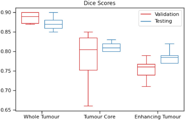
DSC obtained for BraTS 2020 validation and testing datasets

Similarly, a box plot representing the maximum and minimum range of HD95 values was obtained for the validation and testing sub-sets of the BraTS 2020 dataset, as shown in Fig. 13.

Fig. 13.

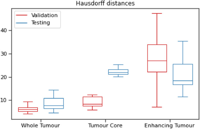
HD95 obtained for BraTS 2020 validation and testing datasets

The complete count of techniques and their accuracy for OS prediction using validation and testing sub-sets of the BraTS 2020 dataset are shown with the help of a bar chart in Figs. 14 and 15, respectively, where the dash (–) symbol represents ‘not given’ entries.

Fig. 14.

SP accuracies obtained for BraTS 2020 validation dataset

Fig. 15.

SP accuracies obtained for BraTS 2020 testing dataset

Research gaps and findings

Even the most advanced algorithms have certain flaws, including the inability to investigate the effect of alternative scanners, protocols, sequences, and dataset sizes, resulting in limited usefulness in regular clinical practice. The segmentation of gliomas is a prerequisite for predicting the survival of the patient. Due to the histological complexity of gliomas, automatic segmentation is not so precise, which affects the SP task as well. From the literature review of SP based on glioma segmentation, it is evident that several research challenges need to be more focused on, which are summarized in Fig. 16.

Fig. 16.

Future research directions for BTS and OS prediction

The research gaps and findings of the existing techniques are explained below:

• Limited training data: A large amount of well-annotated training data are required to build deep generalized models successfully. However, it is a tough job to acquire high-quality, labelled ground-truth data in medical imaging. The patient’s medical information is not publicly available due to ethical barriers and privacy protection. To combat the limited size of publicly available medical datasets, techniques like data augmentation can generate synthetic training examples. Thus, the generation of artificial medical images is still an unexplored research pathway in the literature [113, 117–120]. To understand the tumour heterogeneity more clearly, advanced imaging techniques, such as perfusion-weighted imaging (PWI) and diffusion tensor imaging (DTI), may be employed [36].

• Network failure: The existing network architectures failed to segregate the tumour for several HGG and LGG scans. The networks failed because of the tiny size of the whole tumour, the small size of the NCR, and the absence/small volume of ET. If NCR was not recognised from the raw MRI scans, then during feature extraction model marks all features zero except age due to network failure. In LGG situations, a smaller subcomponent size was observed [33].

• Difficult model training: Researchers have encountered optimization difficulties, such as overfitting, vanishing or exploding gradients, and slow convergence speed while training 3D deep models. High-dimensional 3D data require many parameters, massive memory utilization, and GPU processing to capture more characteristic features. There is a necessity for proper hyperparameter tuning to obtain the best model performance [121–124]. The number of network parameters grows in proportion to the network's depth, require more memory and time to fine-tune them on each epoch [14].

• Overfitting: The technique is prone to overfitting because the training set is minimal [34]. The number of OS individuals examined is less than those of segmentation issues. With a smaller training dataset, the methods cannot extract meaningful information [30]. The trained model's poor performance on unseen patient data demonstrated its overfits to the training dataset [33]. Overfitting is a frequent issue with DNN-based approaches. It may arise owing to a lack of a sufficient quantity of labelled training data for BTS. Overfitting may be addressed by decreasing network complexity (network layers and parameters) or by producing extensive training data utilising image augmentation methods. Augmentation methods generate new images by manipulating input data and their associated ground-truth labels [14].

• Worst tumour sub-regions to segment: Miron et al. [34] found that the worst score was achieved on the ET segmentation, which appears to still suffer from false positives, consistent with other researchers' findings in the challenge. When researchers compared the mean outcomes of subregion segment scores for datasets, they discovered that the ET segment performed poorly [30]. While some segmentation methods performed well in ET and TC, they performed poorly in WT. It means that the models did not do well when it came to categorising ED labels. It was also apparent from the DSC median values, where the median DSC for TC was more significant than the WT [41].

• LGG cases: There are certain outlier instances whereby performance has declined [30]. The overall performance of suggested solutions was outstanding in more than half of the instances, and researchers believed that the LGG examples decreased the mean values. The increased ET sensitivity values demonstrated that the models had missed a small number of ET occurrences [41]. Training LGGs and HGGs separately have been found to improve performance. When it comes to testing, though, this information is not readily accessible. Instead of a distinct boundary between the TC and the surrounding ED, LGGs often exhibit a gradual reduction in tumour-cell density [125].

• Feature selection: As a result of utilising radiomic characteristics, the authors had achieved unsatisfactory performance. Many characteristics were initially retrieved, resulting in a tough time choosing the most important ones, which may explain the problem. The robustness and repeatability of the feature selection method must be evaluated in future research [29]. Due to a variety of network characteristics, normalisation has a minimal impact [30]. Due to its reduced fluctuation inaccuracy, PCA was selected for processing high-dimensional data [45]. Adding more characteristics to the radiomics model may improve its performance on unknown sets [36]. The maximum reported accuracy for the SP task is less than 63% [14]. The dependency of the SP feature extraction step on segmented tumour labels can affect the complete survival prognosis outcome. The biological significance of the retrieved characteristics is also significant. The SP cannot be accurate if the significance of the characteristics is not adequately understood.

• Class biasness: MRI volumes can be segmented through DL techniques, but this is becoming complicated due to highly imbalanced data. In the case of LGG, this class imbalance is more serious. The segmentation networks do not perform well with LGG volumes. Data with large-class variance or inadequate variation contribute to poor performance in the processing of medical images. The segmentation classes are highly asymmetric. For a sample brain tumour MRI slice, about 98% of the voxels belong to either healthy tissue or the surrounding black region, 1.02% belong to the ED class, 0.29% belong to the ET class, and 0.23% belong to the NCR/NET class [94, 126]. The class imbalance may be dealt with via appropriate training data sampling, better loss functions, and augmentation methods. There are only a few survival models that can forecast mid-survivors. It indicates that separating among three classes is more complicated than just separating between two.

• Model generalization: Cross-validation could not generalise the networks even after considering very few parameters [30]. When comparing official validation and testing data, it is essential to note that OS MSE increased significantly, while accuracy did not decrease as much. Further research on the OS multiproblem is required [31]. The model’s generalizability can be enhanced by identifying architectural improvements [35]. The use of traditional linear regression models for OS prediction provides superior results due to their robustness and generalizability [36].

• Non-consistent performance: There is a more considerable performance difference in OS prediction than BTS [46]. The performance obtained on the training set was not preserved on the testing set. The researchers found that normalisation based on normal healthy brain sub-regions reduced the DSC values for the segmentation model when no prior knowledge was used. Ultimately, such normalization approaches did not result in consistency on unseen data [78].

Conclusion and discussion

Because of the benchmark BraTS dataset, the domain of automated medical image analysis for BTS and OS prediction has expanded. The article offers a thorough assessment of the literature on SP techniques presented in the BraTS 2020 Challenge. The critical points are concluded as below:

• Essential steps: The pre-processing, patch selection, loss functions, and post-processing are critical for the network's robust performance [33]. It also implies that if the overall performance is excellent, further increasing patch size and improved validation results may improve the model’s performance on unseen data. Altering training methods and expanding the feature collection may improve the accuracy [30]. The addition of boundary-reweighted cross-entropy improves HD95 and DSC for all sub-regions [35]. Compared to the conventional learning process of the DCNN model, spherical coordinate transformation-based pre-processing help explore data differently by altering the learning process and obtaining new features. These features can assist in segmentation and deep feature extraction for patients' OS prediction. Merging Spherical model labels with the Cartesian models’ WT label filter enhances the segmentation results of all classes [45].

• 2D and 3D: The effectiveness of 2.5D models was inferior to that of 3D models; however, combining both the designs enhances the ensemble's overall performance [29]. The 3D models provide depth information, while the 2D models correctly hyper-tune model parameters and improve the overall performance [41]. Though 2D network techniques require less computer resources and computation time, the apparent benefits of 3D neural architectures and ensemble designs demonstrate a performance difference in tumour segmentation between both the 2D network-based strategy and the 3D network-based strategy [46].

• CNN: All CNN models get overfitted within a few epochs, regardless of the number of layers in the model; thus, it confirms the need for additional training data for the model to learn. A deep learning method, on the other hand, yielded a higher SpearmanR coefficient and reduced the error. CNN models were compared to feature-based models that were handcrafted. Several CNN architectures with many model parameters outperformed biophysical characteristics and age-based models [29]. Given the present state of research, it raises the concern that generic DL interpretation models for OS prediction have limited performance [46].

• UNet-based architectures: The tumour segmentation issue showed that the generic UNet, when combined with carefully chosen pre-processing techniques followed by hyperparameters, outperformed the state-of-the-art on BTS [36]. The visualisation of attention maps revealed that UNets focused more on the tumour region. Loss application seems to have better-optimized segmentation results obtained from the UNet when combined with the gradients obtained from survival models. T-EDet outperformed the UNet 3D core alone in terms of performance. Further research into T-EDet, or perhaps combining 3D and 2D techniques, may result in even more outstanding performance in future studies [31].

• Effective techniques: Researchers believe that using transfer learning to match volumetric data from 3D models with 2D slice-wise predictions is the best way forward [31]. They used a co-training method to enhance the UNet's effectiveness in segmenting ET [36]. The coarse-to-fine approach may substantially increase DSC while decreasing HD95 [95]. During training, the network used the hard mining phase to generate complicated learning instances [32]. MRI scans were identified even in unfavourable lighting and noise by utilising neuromorphic NNs since these networks need very few variables that require adjustment according to the available mMRI data [46]. The findings demonstrated the efficacy of brain parcellation as an extra input. Additional characteristics derived from brain parcellation may improve SP accuracy. One likely drawback is that the brain parcellation may be incorrect around the tumour areas due to intensity fluctuations [95].

• Post-processing: Even though the TC class DSC dropped and the WT class did not improve further, post-processing the segmented region generated using both Cartesian as well as Spherical transformation architectures resulted in the maximum overall improvement on ET [45]. In post-processing, false-positive segmentation voxels are eliminated [33]. It is apparent that post-processing substantially improved the model's efficiency on the BraTS dataset [36]. Further, it was discovered that for certain LGG, the TC was unidentified, and the smaller portions of the solid tumour were properly separated, but the bulk was not. Minimizing the segmentation threshold from 0.5 to 0.05 resulted in properly segmented solid tumours along with numerous false-positive TC identifications in HGGs [37].

• Regression then classification approach: This suggests that a combination of classification and regression helps solve the prediction issue [95]. If the classification model predicted a different class with greater probability than the regression model, the projected survival time would be the output of that model in order to improve resilience. A set survival period of 10 or 15 months was used instead of the anticipated OS in this instance. This combination of prediction and classification is considered innovative by researchers [37].

• Importance of age and gender: A strong correlation exists between age and survival prognosis on the training set [29]. Patient age alone has been proven to be a good predictor of patient prognosis, outperforming more complex radiomic characteristics [37]. According to the research [127], gender also affects tumour therapy. As a result, females have a longer life expectancy than males. It is possible to enhance OS correctness [33] by including the 'gender' feature in the current list.

• Fusion: Features-level fusion and decision-level fusion are the two information fusion techniques that improve classifier performance. It is possible to build an accurate OS time prediction model using a basic NN by integrating various image feature extraction techniques [69]. Ensemble models are used for decision-level fusion because these models combine output prediction probabilities from many to produce a single output prediction probability, which means that local and global knowledge may be combined beneficially.

• Molecular features: Indeed, the most recent WHO classification included molecular gliomas as well as the evaluation of IDH status for diffuse astrocytomas and GBM, as well as 1p/19q co-deletion for oligodendroglioma [8]. These molecular features are required for tumour diagnosis and survival prediction, but they are not included in the BraTS dataset.

Future research directions

Various methods have been suggested to enhance the OS time prediction system. Data denoising methods for MRI pre-processing, raising the complexity of the DL model to learn more semantic features for glioma segmentation, and employing multi-loss functions to handle class imbalance may be used to improve the segmentation performance. ML models trained on texture characteristics derived through a co-occurrence matrix may enhance the SP classification results [69]. Future work will also include surface and volume attributes as a part of the embedded statistics of SP branches [38]. Investigations are required to bridge the difference between the existing GBM radiomics research outside of BraTS, which promotes intensity-based features concerning normalisation methods to benefit from the additional intensity information in a multi-centre environment and the relevant details in pre-treatment MRI about the OS. Because the therapy procedure and some other critical factors, such as methylation status, are unknown in the BraTS dataset, it anticipates achieving a strict performance based on the limited available data. A subset of the BraTS dataset was collected before the latest imaging guidelines, and treatment practises, so studying how this affects the relevance of models built from BraTS data to actual clinical data will be very beneficial [78]. The researchers want to fully evaluate the usage of spatial dropout layers, determining where such dropout layers should be put inside the network and with what proportion these should be used. They plan to evaluate the effectiveness of more complex techniques of test-time augmentation. They also want to investigate Generative Adversarial Networks (GANs) to augment data during training [35]. In future, by integrating atlas-based techniques with DL to get a more precise brain parcellation, the accuracy of BTS and SP techniques can be further improved [95]. The future research directions are also presented in Fig. 17.

Fig. 17.

Future research directions for BTS and OS prediction

Abbreviations

AE

Accumulated encoder

ANN

Artificial neural network

AUNet

Asymmetric UNet

ARD

Automatic relevance determination regression

BN

Batch normalization

BiFPN

Bi-directional feature pyramid network

BTS

Brain tumour segmentation

CNS

Central nervous system

CBICA

Centre for biomedical image computing and analytics

CSF

Cerebrospinal fluid

CN

Channel normalization

CHSQ

Chisquare score

CSV

Comma separated value

CIFE

Conditional infomax feature extraction

CMIM

Conditional mutual information maximization

CRF

Conditional random field

CCA

Connected component analysis

CNN

Convolutional neural network

DT

Decision tree

DCNN

Deep convolutional neural network

DL

Deep learning

DNN

Deep neural network

DSC

Dice similarity coefficient

DTI

Diffusion tensor imaging

DMFNet

Dilated multi-fiber network

DISR

Double input symmetric relevance

ED

Edema

EffUNet

Efficient UNet

ET

Enhancing tumour

FMU

Feature mining unit

FSCR

Fischer score

FCNN

Fully convolution neural network

GDL

Generalized dice loss

GLM

Generalized linear model

GAN

Generative adversarial network

GBM

Glioblastoma multiforme

GPU

Graphical processing unit

GLCM

Gray level co-occurrence matrix

GLDM

Gray level dependence matrix

GLRLM

Gray level run length matrix

GLSZM

Gray level size zone matrix

GM

Grey matter

GTR

Gross total resection

GTV

Gross tumour volume

GN

Group normalization

HD95

Hausdorff distance

HGG

High-grade glioma

IN

Instance normalization

ICAP

Interaction capping

ICC

Intraclass correlation coefficient

JMI

Joint mutual information

LoG

Laplacian of Gaussian

LE

Lesion encoder

LGG

Low-grade glioma

ML

Machine learning

MRI

Magnetic Resonance imaging

MRF

Markov random field

MSE

Mean square error

MSD

Mean squared deviation

MICCAI

Medical image computing and computer-assisted intervention

MRMR

Minimum redundancy maximum relevance

MF

MultiFiber

MLP

Multi-layer perceptron

BraTS Challenge

Multimodal brain tumour segmentation challenge

mMRI

Multimodal MRI

MIFS

Mutual information feature selection

MIM

Mutual information maximization

NCR

Necrosis

NGTDM

Neighboring gray tone difference matrix

NN

Neural network

NET

Non-enhancing tumour

NA

Not applicable

OS

Overall survival

PWI

Perfusion-weighted imaging

PCA

Principal component analysis

RF

Random forest

RFR

Random forest regressor

ReLU

Rectifier linear unit

ROI

Region of interest

RIC

Relative invasiveness coefficient

RNC

Relative necrosis coefficient

RELF

ReliefF

STP

Segmentation then prediction

SK

Selective kernel

srUNet

Self-ensemble ResUNet

SNR

Signal-to-noise ratio

STR

Subtotal resection

SVR

Support vector regression

SP

Survival prediction

SyN

Symmetric normalization

T1

T1-weighted MRI

T1ce

T1-weighted MRI with contrast enhancement

T2

T2-weighted MRI

T2 FLAIR

T2-weighted MRI with fluid-attenuated inversion recovery

3D

Three-dimensional

TNR

True negative rate

TPR

True positive rate

TC

Tumour core

T-EDet

Tumour-efficientDet

2D

Two-dimensional

UNet-AT

UNet attention

VAE

Variational auto-encoder

VOI

Volume of interest

WCEL

Weighted cross-entropy loss

WT

Whole tumour

WHO

World Health Organization

Author contributions

GK, PSR, VA: topic selection, conceptualisation. GK, PSR, VA: literature search and review, data analysis. GK, PSR, VA: methodology and content planning. GK, PSR, VA: manuscript drafting—review and editing.

Funding

No funding was received for this work.

Declarations

Conflict of interest

On behalf of all the authors, the corresponding author declares no conflict of interest.

This article does not contain any studies with human or animal subjects performed by any authors.

References

- 1.DeAngelis LM. Brain tumors. N Engl J Med. 2001;344:114–123. doi: 10.1056/NEJM200101113440207. [DOI] [PubMed] [Google Scholar]
- 2.Ostrom QT, Patil N, Cioffi G, Waite K, Kruchko C, Barnholtz-Sloan JS. CBTRUS statistical report: primary brain and other central nervous system tumors diagnosed in the United States in 2013–2017. Neuro Oncol. 2020;22:1–96. doi: 10.1093/neuonc/noaa200. [DOI] [PMC free article] [PubMed] [Google Scholar]
- 3.Hanif F, Muzaffar K, Perveen K, Malhi SM, Simjee SU. Glioblastoma multiforme: a review of its epidemiology and pathogenesis through clinical presentation and treatment. Asian Pac J Cancer Prev. 2017;18:3–9. doi: 10.22034/APJCP.2017.18.1.3. [DOI] [PMC free article] [PubMed] [Google Scholar]
- 4.Ellor SV, Pagano-Young TA, Avgeropoulos NG. Glioblastoma: background, standard treatment paradigms, and supportive care considerations. J Law Med Ethics. 2014;42:171–182. doi: 10.1111/jlme.12133. [DOI] [PubMed] [Google Scholar]
- 5.Shboul ZA, Alam M, Vidyaratne L, Pei L, Elbakary MI, Iftekharuddin KM. Feature-guided deep radiomics for glioblastoma patient survival prediction. Front Neurosci. 2019;13:966. doi: 10.3389/fnins.2019.00966. [DOI] [PMC free article] [PubMed] [Google Scholar]
- 6.Menze BH, Jakab A, Bauer S, Kalpathy-Cramer J, Farahani K, Kirby J, Burren Y, Porz N, Slotboom J, Wiest R, Lanczi L, Gerstner E, Weber M-A, Arbel T, Avants BB, Ayache N, Buendia P, Collins DL, Cordier N, Corso JJ, Criminisi A, Das T, Delingette H, Demiralp Ç, Durst CR, Dojat M, Doyle S, Festa J, Forbes F, Geremia E, Glocker B, Golland P, Guo X, Hamamci A, Iftekharuddin KM, Jena R, John NM, Konukoglu E, Lashkari D, Mariz JA, Meier R, Pereira S, Precup D, Price SJ, Raviv TR, Reza SMS, Ryan M, Sarikaya D, Schwartz L, Shin H-C, Shotton J, Silva CA, Sousa N, Subbanna NK, Szekely G, Taylor TJ, Thomas OM, Tustison NJ, Unal G, Vasseur F, Wintermark M, Ye DH, Zhao L, Zhao B, Zikic D, Prastawa M, Reyes M, Van Leemput K. The multimodal brain tumor image segmentation benchmark (BRATS) IEEE Trans Med Imaging. 2015;34:1993–2024. doi: 10.1109/TMI.2014.2377694. [DOI] [PMC free article] [PubMed] [Google Scholar]
- 7.Akbari H, Macyszyn L, Da X, Wolf RL, Bilello M, Verma R, O’Rourke DM, Davatzikos C. Pattern analysis of dynamic susceptibility contrast-enhanced MR imaging demonstrates peritumoral tissue heterogeneity. Radiology. 2014;273:502–510. doi: 10.1148/radiol.14132458. [DOI] [PMC free article] [PubMed] [Google Scholar]
- 8.Louis DN, Perry A, Reifenberger G, von Deimling A, Figarella-Branger D, Cavenee WK, Ohgaki H, Wiestler OD, Kleihues P, Ellison DW. The World Health Organization classification of tumors of the central nervous system: a summary. Acta Neuropathol. 2016;131(2016):803–820. doi: 10.1007/s00401-016-1545-1. [DOI] [PubMed] [Google Scholar]
- 9.Stupp R, Mason WP, van den Bent MJ, Weller M, Fisher B, Taphoorn MJB, Belanger K, Brandes AA, Marosi C, Bogdahn U, Curschmann J, Janzer RC, Ludwin SK, Gorlia T, Allgeier A, Lacombe D, Cairncross JG, Eisenhauer E, Mirimanoff RO. Radiotherapy plus concomitant and adjuvant temozolomide for glioblastoma. N Engl J Med. 2005;352:987–996. doi: 10.1056/NEJMoa043330. [DOI] [PubMed] [Google Scholar]
- 10.Weller M, van den Bent M, Tonn JC, Stupp R, Preusser M, Cohen-Jonathan-Moyal E, Henriksson R, Rhun EL, Balana C, Chinot O, Bendszus M, Reijneveld JC, Dhermain F, French P, Marosi C, Watts C, Oberg I, Pilkington G, Baumert BG, Taphoorn MJB, Hegi M, Westphal M, Reifenberger G, Soffietti R, Wick W. European Association for Neuro-Oncology (EANO) guideline on the diagnosis and treatment of adult astrocytic and oligodendroglial gliomas. Lancet Oncol. 2017;18:e315–e329. doi: 10.1016/S1470-2045(17)30194-8. [DOI] [PubMed] [Google Scholar]
- 11.Eckel-Passow JE, Lachance DH, Molinaro AM, Walsh KM, Decker PA, Sicotte H, Pekmezci M, Rice T, Kosel ML, Smirnov IV, Sarkar G, Caron AA, Kollmeyer TM, Praska CE, Chada AR, Halder C, Hansen HM, McCoy LS, Bracci PM, Marshall R, Zheng S, Reis GF, Pico AR, O’Neill BP, Buckner JC, Giannini C, Huse JT, Perry A, Tihan T, Berger MS, Chang SM, Prados MD, Wiemels J, Wiencke JK, Wrensch MR, Jenkins RB (2015) Glioma groups based on 1p/19q, IDH, and TERT promoter mutations in tumors. https://www.nejm.org/doi/10.1056/NEJMoa1407279. Accessed 18 Sept 2021
- 12.Onishi M, Ichikawa T, Kurozumi K, Date I. Angiogenesis and invasion in glioma. Brain Tumor Pathol. 2011;28:13–24. doi: 10.1007/s10014-010-0007-z. [DOI] [PubMed] [Google Scholar]
- 13.Brain Tumor-Grades and Prognostic Factors, Cancer.Net (2012) https://www.cancer.net/cancer-types/brain-tumor/grades-and-prognostic-factors. Accessed 18 Sept 2021
- 14.Agravat RR, Raval MS. A survey and analysis on automated glioma brain tumor segmentation and overall patient survival prediction. Arch Computat Methods Eng. 2021;28:4117–4152. doi: 10.1007/s11831-021-09559-w. [DOI] [Google Scholar]
- 15.Leung D, Han X, Mikkelsen T, Nabors LB. Role of MRI in primary brain tumor evaluation. J Natl Compr Canc Netw. 2014;12:1561–1568. doi: 10.6004/jnccn.2014.0156. [DOI] [PubMed] [Google Scholar]
- 16.Gordillo N, Montseny E, Sobrevilla P. State of the art survey on MRI brain tumor segmentation. Magn Reson Imaging. 2013;31:1426–1438. doi: 10.1016/j.mri.2013.05.002. [DOI] [PubMed] [Google Scholar]
- 17.Chang K, Beers AL, Bai HX, Brown JM, Ly KI, Li X, Senders JT, Kavouridis VK, Boaro A, Su C, Bi WL, Rapalino O, Liao W, Shen Q, Zhou H, Xiao B, Wang Y, Zhang PJ, Pinho MC, Wen PY, Batchelor TT, Boxerman JL, Arnaout O, Rosen BR, Gerstner ER, Yang L, Huang RY, Kalpathy-Cramer J. Automatic assessment of glioma burden: a deep learning algorithm for fully automated volumetric and bidimensional measurement. Neuro Oncol. 2019;21:1412–1422. doi: 10.1093/neuonc/noz106. [DOI] [PMC free article] [PubMed] [Google Scholar]
- 18.Beig N, Patel J, Prasanna P, Hill V, Gupta A, Correa R, Bera K, Singh S, Partovi S, Varadan V, Ahluwalia M, Madabhushi A, Tiwari P. Radiogenomic analysis of hypoxia pathway is predictive of overall survival in Glioblastoma. Sci Rep. 2018;8:7. doi: 10.1038/s41598-017-18310-0. [DOI] [PMC free article] [PubMed] [Google Scholar]
- 19.Chang K, Bai HX, Zhou H, Su C, Bi WL, Agbodza E, Kavouridis VK, Senders JT, Boaro A, Beers A, Zhang B, Capellini A, Liao W, Shen Q, Li X, Xiao B, Cryan J, Ramkissoon S, Ramkissoon L, Ligon K, Wen PY, Bindra RS, Woo J, Arnaout O, Gerstner ER, Zhang PJ, Rosen BR, Yang L, Huang RY, Kalpathy-Cramer J. Residual convolutional neural network for the determination of IDH status in low- and high-grade gliomas from MR imaging. Clin Cancer Res. 2018;24:1073–1081. doi: 10.1158/1078-0432.CCR-17-2236. [DOI] [PMC free article] [PubMed] [Google Scholar]
- 20.White N, Reid F, Harris A, Harries P, Stone P. A Systematic review of predictions of survival in palliative care: how accurate are clinicians and who are the experts? PLoS ONE. 2016;11:e0161407. doi: 10.1371/journal.pone.0161407. [DOI] [PMC free article] [PubMed] [Google Scholar]
- 21.Lao J, Chen Y, Li Z-C, Li Q, Zhang J, Liu J, Zhai G. A deep learning-based radiomics model for prediction of survival in glioblastoma multiforme. Sci Rep. 2017;7:10353. doi: 10.1038/s41598-017-10649-8. [DOI] [PMC free article] [PubMed] [Google Scholar]
- 22.Bakas S, Akbari H, Sotiras A, Bilello M, Rozycki M, Kirby JS, Freymann JB, Farahani K, Davatzikos C. Advancing the cancer genome atlas glioma MRI collections with expert segmentation labels and radiomic features. Sci Data. 2017;4:170117. doi: 10.1038/sdata.2017.117. [DOI] [PMC free article] [PubMed] [Google Scholar]
- 23.Bakas S, Reyes M, Jakab A et al (2019) Identifying the best machine learning algorithms for brain tumor segmentation, progression assessment, and overall survival prediction in the BRATS challenge. ArXiv:1811.02629 [Cs, Stat]. http://arxiv.org/abs/1811.02629. Accessed 18 Sept 2021
- 24.Bakas S, Akbari H, Sotiras A, Bilello M, Rozycki M, Kirby J, Freymann J, Farahani K, Davatzikos C (2017) Segmentation labels for the pre-operative scans of the TCGA-GBM collection. The Cancer Imaging Archive. https://wiki.cancerimagingarchive.net/x/KoZyAQ. Accessed 22 July 2021
- 25.Bakas S, Akbari H, Sotiras A, Bilello M, Rozycki M, Kirby J, Freymann J, Farahani K, Davatzikos C (2017) Segmentation labels for the pre-operative scans of the TCGA-LGG collection. The Cancer Imaging Archive. https://wiki.cancerimagingarchive.net/x/LIZyAQ. Accessed 22 July 2021
- 26.Havaei M, Davy A, Warde-Farley D, Biard A, Courville A, Bengio Y, Pal C, Jodoin P-M, Larochelle H. Brain tumor segmentation with deep neural networks. Med Image Anal. 2017;35:18–31. doi: 10.1016/j.media.2016.05.004. [DOI] [PubMed] [Google Scholar]
- 27.Kamnitsas K, Ledig C, Newcombe VFJ, Simpson JP, Kane AD, Menon DK, Rueckert D, Glocker B. Efficient multi-scale 3D CNN with fully connected CRF for accurate brain lesion segmentation. Med Image Anal. 2017;36:61–78. doi: 10.1016/j.media.2016.10.004. [DOI] [PubMed] [Google Scholar]
- 28.Pereira S, Pinto A, Alves V, Silva CA. Brain tumor segmentation using convolutional neural networks in MRI images. IEEE Trans Med Imaging. 2016;35:1240–1251. doi: 10.1109/TMI.2016.2538465. [DOI] [PubMed] [Google Scholar]
- 29.González SR, Zemmoura I, Tauber C (2021) 3D brain tumor segmentation and survival prediction using ensembles of convolutional neural networks. In: Brainlesion: glioma, multiple sclerosis, stroke and traumatic brain injuries. Springer, Cham, p 241–254. 10.1007/978-3-030-72087-2_21
- 30.Parmar B, Parikh M. brain tumor segmentation and survival prediction using patch based modified 3D U-Net. In: Crimi A, Bakas S, editors. Brainlesion: glioma, multiple sclerosis, stroke and traumatic brain injuries. Cham: Springer; 2021. pp. 398–409. [Google Scholar]
- 31.Carmo D, Rittner L, Lotufo R. MultiATTUNet: brain tumor segmentation and survival multitasking. In: Crimi A, Bakas S, editors. Brainlesion: glioma, multiple sclerosis, stroke and traumatic brain injuries. Cham: Springer; 2021. pp. 424–434. [Google Scholar]
- 32.Anand VK, Grampurohit S, Aurangabadkar P, Kori A, Khened M, Bhat RS, Krishnamurthi G. Brain tumor segmentation and survival prediction using automatic hard mining in 3D CNN architecture. In: Crimi A, Bakas S, editors. Brainlesion: glioma, multiple sclerosis, stroke and traumatic brain injuries. Cham: Springer; 2021. pp. 310–319. [Google Scholar]
- 33.Agravat RR, Raval MS. 3D semantic segmentation of brain tumor for overall survival prediction. In: Crimi A, Bakas S, editors. Brainlesion: glioma, multiple sclerosis stroke and traumatic brain injuries. Cham: Springer; 2021. pp. 215–227. [Google Scholar]
- 34.Miron R, Albert R, Breaban M. A two-stage atrous convolution neural network for brain tumor segmentation and survival prediction. In: Crimi A, Bakas S, editors. Brainlesion: glioma, multiple sclerosis stroke and traumatic brain injuries. Cham: Springer; 2021. pp. 290–299. [Google Scholar]
- 35.Patel J, Chang K, Hoebel K, Gidwani M, Arun N, Gupta S, Aggarwal M, Singh P, Rosen BR, Gerstner ER, Kalpathy-Cramer J (2021) Segmentation, survival prediction, and uncertainty estimation of gliomas from multimodal 3D MRI using selective kernel networks. In: Brainlesion: glioma, multiple sclerosis, stroke and traumatic brain injuries. Springer, Cham, p 228–240. 10.1007/978-3-030-72087-2_20
- 36.Dai C, Wang S, Raynaud H, Mo Y, Angelini E, Guo Y, Bai W. Self-training for brain tumour segmentation with uncertainty estimation and biophysics-guided survival prediction. In: Crimi A, Bakas S, editors. Brainlesion: glioma, multiple sclerosis stroke and traumatic brain injuries. Cham: Springer; 2021. pp. 514–523. [Google Scholar]
- 37.McKinley R, Rebsamen M, Dätwyler K, Meier R, Radojewski P, Wiest R. Uncertainty-driven refinement of tumor-core segmentation using 3D-to-2D networks with label uncertainty. In: Crimi A, Bakas S, editors. Brainlesion: glioma, multiple sclerosis, stroke and traumatic brain injuries. Cham: Springer; 2021. pp. 401–411. [Google Scholar]
- 38.Zhao G, Jiang B, Zhang J, Xia Y. Segmentation then prediction: a multi-task solution to brain tumor segmentation and survival prediction. In: Crimi A, Bakas S, editors. Brainlesion: glioma, multiple sclerosis, stroke and traumatic brain injuries. Cham: Springer; 2021. pp. 492–502. [Google Scholar]
- 39.Pei L, Murat AK, Colen R. Multimodal brain tumor segmentation and survival prediction using a 3D self-ensemble ResUNet. In: Crimi A, Bakas S, editors. Brainlesion: glioma, multiple sclerosis, stroke and traumatic brain injuries. Cham: Springer; 2021. pp. 367–375. [Google Scholar]
- 40.Soltaninejad M, Pridmore T, Pound M. Efficient MRI brain tumor segmentation using multi-resolution encoder-decoder networks. In: Crimi A, Bakas S, editors. Brainlesion: glioma, multiple sclerosis, stroke and traumatic brain injuries. Cham: Springer; 2021. pp. 30–39. [Google Scholar]
- 41.Ali MJ, Akram MT, Saleem H, Raza B, Shahid AR. Glioma segmentation using ensemble of 2D/3D U-Nets and survival prediction using multiple features fusion. In: Crimi A, Bakas S, editors. Brainlesion: glioma, multiple sclerosis, stroke and traumatic brain injuries. Cham: Springer; 2021. pp. 189–199. [Google Scholar]
- 42.Akbar AS, Fatichah C, Suciati N. Modified MobileNet for patient survival prediction. In: Crimi A, Bakas S, editors. Brainlesion: glioma, multiple sclerosis, stroke and traumatic brain injuries. Cham: Springer; 2021. pp. 374–387. [Google Scholar]
- 43.Pang E, Shi W, Li X, Wu Q. Glioma segmentation using encoder-decoder network and survival prediction based on cox analysis. In: Crimi A, Bakas S, editors. Brainlesion: glioma, multiple sclerosis, stroke and traumatic brain injuries. Cham: Springer; 2021. pp. 318–326. [Google Scholar]
- 44.Tustison NJ, Avants BB, Cook PA, Zheng Y, Egan A, Yushkevich PA, Gee JC. N4ITK: improved N3 bias correction. IEEE Trans Med Imaging. 2010;29:1310–1320. doi: 10.1109/TMI.2010.2046908. [DOI] [PMC free article] [PubMed] [Google Scholar]
- 45.Russo C, Liu S, Di Ieva A. Impact of spherical coordinates transformation pre-processing in deep convolution neural networks for brain tumor segmentation and survival prediction. In: Crimi A, Bakas S, editors. Brainlesion: glioma, multiple sclerosis, stroke and traumatic brain injuries. Cham: Springer; 2021. pp. 295–306. [Google Scholar]
- 46.Han IS. Multimodal brain image analysis and survival prediction using neuromorphic attention-based neural networks. In: Crimi A, Bakas S, editors. Brainlesion: glioma, multiple sclerosis, stroke and traumatic brain injuries. Cham: Springer; 2021. pp. 194–206. [Google Scholar]
- 47.Han W-S, Han IS (2020) Multimodal brain image segmentation and analysis with neuromorphic attention-based learning. In: Brainlesion: glioma, multiple sclerosis, stroke and traumatic brain injuries. Springer, Cham, p 14–26. 10.1007/978-3-030-46643-5_2
- 48.Nalepa J, Marcinkiewicz M, Kawulok M. Data augmentation for brain-tumor segmentation: a review. Front Comput Neurosci. 2019;13:83. doi: 10.3389/fncom.2019.00083. [DOI] [PMC free article] [PubMed] [Google Scholar]
- 49.Marti Asenjo J, Martinez-Larraz Solís A. mri brain tumor segmentation using a 2D–3D U-Net ensemble. In: Crimi A, Bakas S, editors. Brainlesion: glioma, multiple sclerosis, stroke and traumatic brain injuries. Cham: Springer; 2021. pp. 354–366. [Google Scholar]
- 50.Wang L, Wang S, Chen R, Qu X, Chen Y, Huang S, Liu C. Nested dilation networks for brain tumor segmentation based on magnetic resonance imaging. Front Neurosci. 2019;13:285. doi: 10.3389/fnins.2019.00285. [DOI] [PMC free article] [PubMed] [Google Scholar]
- 51.Litjens G, Kooi T, Bejnordi BE, Setio AAA, Ciompi F, Ghafoorian M, van der Laak JAWM, van Ginneken B, Sánchez CI. A survey on deep learning in medical image analysis. Med Image Anal. 2017;42:60–88. doi: 10.1016/j.media.2017.07.005. [DOI] [PubMed] [Google Scholar]
- 52.Sudre CH, Li W, Vercauteren T, Ourselin S, Jorge Cardoso M. generalised dice overlap as a deep learning loss function for highly unbalanced segmentations. In: Cardoso MJ, Arbel T, Carneiro G, Syeda-Mahmood T, Tavares JMRS, Moradi M, Bradley A, Greenspan H, Papa JP, Madabhushi A, Nascimento JC, Cardoso JS, Belagiannis V, Lu Z, editors. Deep learning in medical image analysis and multimodal learning for clinical decision support. Cham: Springer; 2017. pp. 240–248. [DOI] [PMC free article] [PubMed] [Google Scholar]
- 53.Chen C, Liu X, Ding M, Zheng J, Li J. Medical image computing and computer assisted intervention—MICCAI 2019. Cham: Springer; 2019. 3D dilated multi-fiber network for real-time brain tumor segmentation in MRI; pp. 184–192. [Google Scholar]
- 54.Isensee F, Kickingereder P, Wick W, Bendszus M, Maier-Hein KH. Brain tumor segmentation and radiomics survival prediction: contribution to the BRATS 2017 challenge. In: Crimi A, Bakas S, Kuijf H, Menze B, Reyes M, editors. Brainlesion: glioma, multiple sclerosis, stroke and traumatic brain injuries. Cham: Springer; 2018. pp. 287–297. [Google Scholar]
- 55.Jiang Z, Ding C, Liu M, Tao D (2020) Two-stage cascaded U-Net: 1st place solution to BraTS challenge 2019 segmentation task. In: Brainlesion: glioma, multiple sclerosis, stroke and traumatic brain injuries. Springer, Cham, p 231–241. 10.1007/978-3-030-46640-4_22
- 56.Myronenko A (2019) 3D MRI brain tumor segmentation using autoencoder regularization. In: Brainlesion: glioma, multiple sclerosis, stroke and traumatic brain injuries. Springer, Cham, p 311–320. 10.1007/978-3-030-11726-9_28
- 57.Zhou C, Ding C, Lu Z, Wang X, Tao D. One-pass multi-task convolutional neural networks for efficient brain tumor segmentation. In: Frangi AF, Schnabel JA, Davatzikos C, Alberola-López C, Fichtinger G, editors. Medical image computing and computer assisted intervention—MICCAI 2018. Cham: Springer; 2018. pp. 637–645. [Google Scholar]
- 58.Agravat RR, Raval MS. Chapter 11—Deep learning for automated brain tumor segmentation in MRI images. In: Dey N, Ashour AS, Shi F, Balas VE, editors. Soft computing based medical image analysis. New York: Academic Press; 2018. pp. 183–201. [Google Scholar]
- 59.Ronneberger O, Fischer P, Brox T (2015) U-Net: convolutional networks for biomedical image segmentation, in: medical image computing and computer-assisted intervention—MICCAI 2015, Springer, Cham, p 234–241. 10.1007/978-3-319-24574-4_28
- 60.Milletari F, Navab N, Ahmadi S-A (2016) V-Net: fully convolutional neural networks for volumetric medical image segmentation. In: 2016 fourth international conference on 3D vision (3DV), p 565–571. 10.1109/3DV.2016.79
- 61.Badrinarayanan V, Kendall A, Cipolla R. SegNet: a deep convolutional encoder-decoder architecture for image segmentation. IEEE Trans Pattern Anal Mach Intell. 2017;39:2481–2495. doi: 10.1109/TPAMI.2016.2644615. [DOI] [PubMed] [Google Scholar]
- 62.He K, Zhang X, Ren S, Sun J (2016) Deep residual learning for image recognition. In: Proceedings of the IEEE conference on computer vision and pattern recognition, p 770–778. https://openaccess.thecvf.com/content_cvpr_2016/html/He_Deep_Residual_Learning_CVPR_2016_paper.html. Accessed 18 Sept 2021
- 63.Iandola F, Moskewicz M, Karayev S, Girshick R, Darrell T, Keutzer K (2014) DenseNet: implementing efficient ConvNet descriptor pyramids. ArXiv:1404.1869 [Cs]. http://arxiv.org/abs/1404.1869. Accessed 18 Sept 2021
- 64.Isensee F, Kickingereder P, Wick W, Bendszus M, Maier-Hein KH. No New-Net. In: Crimi A, Bakas S, Kuijf H, Keyvan F, Reyes M, van Walsum T, editors. Brainlesion: glioma, multiple sclerosis, stroke and traumatic brain injuries. Cham: Springer; 2019. pp. 234–244. [Google Scholar]
- 65.Kamnitsas K, Bai W, Ferrante E, McDonagh S, Sinclair M, Pawlowski N, Rajchl M, Lee M, Kainz B, Rueckert D, Glocker B. Ensembles of multiple models and architectures for robust brain tumour segmentation. In: Crimi A, Bakas S, Kuijf H, Menze B, Reyes M, editors. Brainlesion: glioma, multiple sclerosis, stroke and traumatic brain injuries. Cham: Springer; 2018. pp. 450–462. [Google Scholar]
- 66.McKinley R, Rebsamen M, Meier R, Wiest R (2020) Triplanar ensemble of 3D-to-2D CNNs with label-uncertainty for brain tumor segmentation. In: Brainlesion: glioma, multiple sclerosis, stroke and traumatic brain injuries. Springer, Cham, p 379–387. 10.1007/978-3-030-46640-4_36
- 67.Zhao Y-X, Zhang Y-M, Liu C-L. Bag of tricks for 3D MRI brain tumor segmentation. In: Crimi A, Bakas S, editors. Brainlesion: glioma, multiple sclerosis, stroke and traumatic brain injuries. Cham: Springer; 2020. pp. 210–220. [Google Scholar]
- 68.Myronenko A, Hatamizadeh A. Robust semantic segmentation of brain tumor regions from 3D MRIs. In: Crimi A, Bakas S, editors. Brainlesion: glioma, multiple sclerosis, stroke and traumatic brain injuries. Cham: Springer; 2020. pp. 82–89. [Google Scholar]
- 69.Chato L, Kachroo P, Latifi S. An automatic overall survival time prediction system for glioma brain tumor patients based on volumetric and shape features. In: Crimi A, Bakas S, editors. Brainlesion: glioma, multiple sclerosis, stroke and traumatic brain injuries. Cham: Springer; 2021. pp. 352–365. [Google Scholar]
- 70.Dai Z, Heckel R (2019) Channel normalization in convolutional neural network avoids vanishing gradients. ArXiv:1907.09539 [Cs, Stat]. http://arxiv.org/abs/1907.09539. Accessed 19 Sept 2021
- 71.Ioffe S, Szegedy C (2015) Batch normalization: accelerating deep network training by reducing internal covariate shift. In: International conference on machine learning, PMLR, p 448–456. https://proceedings.mlr.press/v37/ioffe15.html. Accessed 18 Sept 2021
- 72.Khened M, Kori A, Rajkumar H, Krishnamurthi G, Srinivasan B. A generalized deep learning framework for whole-slide image segmentation and analysis. Sci Rep. 2021;11:11579. doi: 10.1038/s41598-021-90444-8. [DOI] [PMC free article] [PubMed] [Google Scholar]
- 73.Szegedy C, Liu W, Jia Y, Sermanet P, Reed S, Anguelov D, Erhan D, Vanhoucke V, Rabinovich A (2015) Going deeper with convolutions. In: 2015 IEEE conference on computer vision and pattern recognition (CVPR), p 1–9. 10.1109/CVPR.2015.7298594
- 74.Szegedy C, Vanhoucke V, Ioffe S, Shlens J, Wojna Z (2016) Rethinking the inception architecture for computer vision. In: Proceedings of the IEEE conference on computer vision and pattern recognition, p 2818–2826. https://www.cv-foundation.org/openaccess/content_cvpr_2016/html/Szegedy_Rethinking_the_Inception_CVPR_2016_paper.html. Accessed 18 Sept 2021
- 75.Iandola FN, Han S, Moskewicz MW, Ashraf K, Dally WJ, Keutzer K (2016) SqueezeNet: AlexNet-level accuracy with 50x fewer parameters and <0.5MB model size. ArXiv:1602.07360 [Cs]. http://arxiv.org/abs/1602.07360. Accessed 19 Sept 2021
- 76.Lin T-Y, Dollár P, Girshick R, He K, Hariharan B, Belongie S (2017) Feature pyramid networks for object detection. ArXiv:1612.03144 [Cs]. http://arxiv.org/abs/1612.03144. Accessed 19 Sept 2021
- 77.Kong X, Sun G, Wu Q, Liu J, Lin F. Hybrid pyramid U-Net model for brain tumor segmentation. In: Shi Z, Mercier-Laurent E, Li J, editors. Intelligent information processing IX. Cham: Springer; 2018. pp. 346–355. [Google Scholar]
- 78.Suter Y, Knecht U, Wiest R, Reyes M (2021) Overall survival prediction for glioblastoma on pre-treatment MRI using robust radiomics and priors. In: Brainlesion: glioma, multiple sclerosis, stroke and traumatic brain injuries. Springer, Cham, p 307–317. 10.1007/978-3-030-72084-1_28
- 79.Jenkinson M, Beckmann CF, Behrens TEJ, Woolrich MW, Smith SM. FSL. Neuroimage. 2012;62:782–790. doi: 10.1016/j.neuroimage.2011.09.015. [DOI] [PubMed] [Google Scholar]
- 80.Isensee F, Petersen J, Klein A, Zimmerer D, Jaeger PF, Kohl S, Wasserthal J, Koehler G, Norajitra T, Wirkert S, Maier-Hein KH (2018) nnU-Net: self-adapting framework for U-net-based medical image segmentation. ArXiv:1809.10486 [Cs]. http://arxiv.org/abs/1809.10486. Accessed 19 Sept 2021
- 81.Wu Y, He K (2018) Group normalization. In: Proceedings of the European conference on computer vision (ECCV), p 3–19. https://openaccess.thecvf.com/content_ECCV_2018/html/Yuxin_Wu_Group_Normalization_ECCV_2018_paper.html. Accessed 18 Sept 2021
- 82.Li X, Wang W, Hu X, Yang J (2019) Selective kernel networks. In: Proceedings of the IEEE/CVF conference on computer vision and pattern recognition, p 510–519. https://openaccess.thecvf.com/content_CVPR_2019/html/Li_Selective_Kernel_Networks_CVPR_2019_paper.html. Accessed 18 Sept 2021
- 83.Kayalibay B, Jensen G, van der Smagt P (2017) CNN-based segmentation of medical imaging data. ArXiv:1701.03056 [Cs]. http://arxiv.org/abs/1701.03056. Accessed 18 Sept 2021
- 84.Woo S, Park J, Lee J-Y, Kweon IS (2018) CBAM: convolutional block attention module. In: Proceedings of the European conference on computer vision (ECCV), p 3–19. https://openaccess.thecvf.com/content_ECCV_2018/html/Sanghyun_Woo_Convolutional_Block_Attention_ECCV_2018_paper.html. Accessed 18 Sept 2021
- 85.Chen L-C, Papandreou G, Kokkinos I, Murphy K, Yuille AL. DeepLab: semantic image segmentation with deep convolutional nets, atrous convolution, and fully connected CRFs. IEEE Trans Pattern Anal Mach Intell. 2018;40:834–848. doi: 10.1109/TPAMI.2017.2699184. [DOI] [PubMed] [Google Scholar]
- 86.Chen L-C, Zhu Y, Papandreou G, Schroff F, Adam H (2018) Encoder-decoder with atrous separable convolution for semantic image segmentation. In: Proceedings of the European conference on computer vision (ECCV), p 801–818. https://openaccess.thecvf.com/content_ECCV_2018/html/Liang-Chieh_Chen_Encoder-Decoder_with_Atrous_ECCV_2018_paper.html. Accessed 18 Sept 2021
- 87.Feng Y-Z, Liu S, Cheng Z-Y, Quiroz JC, Rezazadegan D, Chen P-K, Lin Q-T, Qian L, Liu X-F, Berkovsky S, Coiera E, Song L, Qiu X-M, Cai X-R (2020) Severity assessment and progression prediction of COVID-19 patients based on the lesion encoder framework and chest CT. MedRxiv. 10.1101/2020.08.03.20167007
- 88.Tan M, Le Q (2019) EfficientNet: rethinking model scaling for convolutional neural networks. In: International conference on machine learning, PMLR, p 6105–6114. https://proceedings.mlr.press/v97/tan19a.html. Accessed 18 Sept 2021
- 89.Ramachandran P, Zoph B, Le QV (2017) Searching for activation functions ArXiv:1710.05941 [Cs]. http://arxiv.org/abs/1710.05941. Accessed 19 Sept 2021
- 90.Chollet F (2017) Xception: deep learning with depthwise separable convolutions. p 1251–1258. https://openaccess.thecvf.com/content_cvpr_2017/html/Chollet_Xception_Deep_Learning_CVPR_2017_paper.html. Accessed 19 Sept 2021
- 91.Carmo D, Silva B, Yasuda C, Rittner L, Lotufo R. Hippocampus segmentation on epilepsy and Alzheimer’s disease studies with multiple convolutional neural networks. Heliyon. 2021;7:e06226. doi: 10.1016/j.heliyon.2021.e06226. [DOI] [PMC free article] [PubMed] [Google Scholar]
- 92.Newell A, Yang K, Deng J. Stacked hourglass networks for human pose estimation. In: Leibe B, Matas J, Sebe N, Welling M, editors. Computer vision—ECCV 2016. Cham: Springer; 2016. pp. 483–499. [Google Scholar]
- 93.Ulyanov D, Vedaldi A, Lempitsky V (2017) Instance normalization: the missing ingredient for fast stylization, ArXiv:1607.08022 [Cs]. http://arxiv.org/abs/1607.08022. Accessed 19 Sept 2021
- 94.Rafi A, Ali J, Akram T, Fiaz K, Raza Shahid A, Raza B, Mustafa Madni T (2020) U-Net based glioblastoma segmentation with patient’s overall survival prediction. In: Intelligent computing systems. Springer, Cham, p 22–32. 10.1007/978-3-030-43364-2_3
- 95.Zhang Y, Wu J, Huang W, Chen Y, Wu EdX, Tang X. Utility of brain parcellation in enhancing brain tumor segmentation and survival prediction. In: Crimi A, Bakas S, editors. Brainlesion: glioma, multiple sclerosis, stroke and traumatic brain injuries. Cham: Springer; 2021. pp. 391–400. [Google Scholar]
- 96.Liu Z, Chen L, Tong L, Zhou F, Jiang Z, Zhang Q, Shan C, Wang Y, Zhang X, Li L, Zhou H (2020) Deep learning based brain tumor segmentation: a survey. ArXiv:2007.09479 [Cs, Eess]. http://arxiv.org/abs/2007.09479. Accessed 19 Sept 2021
- 97.Huang G, Liu Z, van der Maaten L, Weinberger KQ (2017) Densely connected convolutional networks. In: Proceedings of the IEEE conference on computer vision and pattern recognition, p 4700–4708. https://openaccess.thecvf.com/content_cvpr_2017/html/Huang_Densely_Connected_Convolutional_CVPR_2017_paper.html. Accessed 18 Sept 2021
- 98.Buitinck L, Louppe G, Blondel M, Pedregosa F, Mueller A, Grisel O, Niculae V, Prettenhofer P, Gramfort A, Grobler J, Layton R, Vanderplas J, Joly A, Holt B, Varoquaux G (2013) API design for machine learning software: experiences from the scikit-learn project. ArXiv:1309.0238 [Cs]. http://arxiv.org/abs/1309.0238. accessed 18 Sept 2021
- 99.Pedregosa F, Varoquaux G, Gramfort A, Michel V, Thirion B, Grisel O, Blondel M, Prettenhofer P, Weiss R, Dubourg V. Scikit-learn: machine learning in python. J Mach Learn Res. 2011;12:2825–2830. [Google Scholar]
- 100.Srivastava N, Hinton G, Krizhevsky A, Sutskever I, Salakhutdinov R. Dropout: a simple way to prevent neural networks from overfitting. J Mach Learn Res. 2014;15:1929–1958. [Google Scholar]
- 101.Deng J, Dong W, Socher R, Li L-J, Li K, Fei-Fei L (2009) ImageNet: a large-scale hierarchical image database. In: 2009 IEEE conference on computer vision and pattern recognition, p 248–255. 10.1109/CVPR.2009.5206848
- 102.Swanson KR, Rostomily RC, Alvord EC. A mathematical modelling tool for predicting survival of individual patients following resection of glioblastoma: a proof of principle. Br J Cancer. 2008;98:113–119. doi: 10.1038/sj.bjc.6604125. [DOI] [PMC free article] [PubMed] [Google Scholar]
- 103.Swanson KR, Bridge C, Murray JD, Alvord EC. Virtual and real brain tumors: using mathematical modeling to quantify glioma growth and invasion. J Neurol Sci. 2003;216:1–10. doi: 10.1016/j.jns.2003.06.001. [DOI] [PubMed] [Google Scholar]
- 104.Han W-S, Han I-S. All weather human detection using neuromorphic visual processing. In: Chen L, Kapoor S, Bhatia R, editors. Intelligent systems for science and information: extended and selected results from the science and information conference 2013. Cham: Springer; 2014. pp. 25–44. [Google Scholar]
- 105.van Griethuysen JJM, Fedorov A, Parmar C, Hosny A, Aucoin N, Narayan V, Beets-Tan RGH, Fillion-Robin J-C, Pieper S, Aerts HJWL. Computational radiomics system to decode the radiographic phenotype. Cancer Res. 2017;77:e104–e107. doi: 10.1158/0008-5472.CAN-17-0339. [DOI] [PMC free article] [PubMed] [Google Scholar]
- 106.Reuter M, Rosas HD, Fischl B. Highly accurate inverse consistent registration: a robust approach. Neuroimage. 2010;53:1181–1196. doi: 10.1016/j.neuroimage.2010.07.020. [DOI] [PMC free article] [PubMed] [Google Scholar]
- 107.Avants BB, Epstein CL, Grossman M, Gee JC. Symmetric diffeomorphic image registration with cross-correlation: evaluating automated labeling of elderly and neurodegenerative brain. Med Image Anal. 2008;12:26–41. doi: 10.1016/j.media.2007.06.004. [DOI] [PMC free article] [PubMed] [Google Scholar]
- 108.Ramien GN, Jaeger PF, Kohl SAA, Maier-Hein KH. Reg R-CNN: lesion detection and grading under noisy labels. In: Greenspan H, Tanno R, Erdt M, Arbel T, Baumgartner C, Dalca A, Sudre CH, Wells WM, Drechsler K, Linguraru MG, Oyarzun Laura C, Shekhar R, Wesarg S, González Ballester MÁ, editors. Uncertainty for safe utilization of machine learning in medical imaging and clinical image-based procedures. Cham: Springer; 2019. pp. 33–41. [Google Scholar]
- 109.Li C, Wang S, Liu P, Torheim T, Boonzaier NR, van Dijken BR, Schönlieb C-B, Markowetz F, Price SJ. Decoding the interdependence of multiparametric magnetic resonance imaging to reveal patient subgroups correlated with survivals. Neoplasia. 2019;21:442–449. doi: 10.1016/j.neo.2019.03.005. [DOI] [PMC free article] [PubMed] [Google Scholar]
- 110.Baldock AL, Ahn S, Rockne R, Johnston S, Neal M, Corwin D, Clark-Swanson K, Sterin G, Trister AD, Malone H, Ebiana V, Sonabend AM, Mrugala M, Rockhill JK, Silbergeld DL, Lai A, Cloughesy T, Ii GMM, Bruce JN, Rostomily RC, Canoll P, Swanson KR. Patient-specific metrics of invasiveness reveal significant prognostic benefit of resection in a predictable subset of gliomas. PLoS ONE. 2014;9:e99057. doi: 10.1371/journal.pone.0099057. [DOI] [PMC free article] [PubMed] [Google Scholar]
- 111.Li C, Wang S, Yan J-L, Torheim T, Boonzaier NR, Sinha R, Matys T, Markowetz F, Price SJ. Characterizing tumor invasiveness of glioblastoma using multiparametric magnetic resonance imaging. J Neurosurg. 2019;132:1465–1472. doi: 10.3171/2018.12.JNS182926. [DOI] [PubMed] [Google Scholar]
- 112.Wang S, Dai C, Mo Y, Angelini E, Guo Y, Bai W. Automatic brain tumour segmentation and biophysics-guided survival prediction. In: Crimi A, Bakas S, editors. Brainlesion: glioma, multiple sclerosis, stroke and traumatic brain injuries. Cham: Springer; 2020. pp. 61–72. [Google Scholar]
- 113.Feng NE, Dou Q, Tustison N, Meyer C (2020) Brain tumor segmentation with uncertainty estimation and overall survival prediction. In: Brainlesion: glioma, multiple sclerosis, stroke and traumatic brain injuries. Springer, Cham, p 304–314. 10.1007/978-3-030-46640-4_29
- 114.Geurts P, Ernst D, Wehenkel L. Extremely randomized trees. Mach Learn. 2006;63:3–42. doi: 10.1007/s10994-006-6226-1. [DOI] [Google Scholar]
- 115.Nelder JA, Wedderburn RWM. Generalized Linear Models. J R Stat Soc Ser A (Gen) 1972;135:370–384. doi: 10.2307/2344614. [DOI] [Google Scholar]
- 116.Górriz M, Antony J, McGuinness K, Giró-i-Nieto X, O’Connor NE (2019) Assessing knee OA severity with CNN attention-based end-to-end architectures. In: International conference on medical imaging with deep learning, PMLR, p 197–214. https://proceedings.mlr.press/v102/gorriz19a.html. Accessed 18 Sept 2021
- 117.Baid U, Talbar S, Rane S, Gupta S, Thakur MH, Moiyadi A, Thakur S, Mahajan A (2019) Deep learning radiomics algorithm for gliomas (DRAG) model: a novel approach using 3D UNET based deep convolutional neural network for predicting survival in gliomas. In: Brainlesion: glioma, multiple sclerosis, stroke and traumatic brain injuries. Springer, Cham, p 369–379. 10.1007/978-3-030-11726-9_33
- 118.Weninger L, Rippel O, Koppers S, Merhof D (2019) Segmentation of brain tumors and patient survival prediction: methods for the BraTS 2018 challenge. In: Brainlesion: glioma, multiple sclerosis, stroke and traumatic brain injuries. Springer, Cham, p 3–12. 10.1007/978-3-030-11726-9_1
- 119.Suter Y, Jungo A, Rebsamen M, Knecht U, Herrmann E, Wiest R, Reyes M. Deep learning versus classical regression for brain tumor patient survival prediction. In: Crimi A, Bakas S, Kuijf H, Keyvan F, Reyes M, van Walsum T, editors. Brainlesion: glioma, multiple sclerosis, stroke and traumatic brain injuries. Cham: Springer; 2019. pp. 429–440. [Google Scholar]
- 120.Guo X, Yang C, Lam PL, Woo PYM, Yuan Y. Domain knowledge based brain tumor segmentation and overall survival prediction. In: Crimi A, Bakas S, editors. Brainlesion: glioma, multiple sclerosis, stroke and traumatic brain injuries. Cham: Springer; 2020. pp. 285–295. [Google Scholar]
- 121.Wang F, Jiang R, Zheng L, Meng C, Biswal B. 3D U-Net based brain tumor segmentation and survival days prediction. In: Crimi A, Bakas S, editors. Brainlesion: glioma, multiple sclerosis, stroke and traumatic brain injuries. Cham: Springer; 2020. pp. 131–141. [Google Scholar]
- 122.Islam M, Jose VJM, Ren H. Glioma prognosis: segmentation of the tumor and survival prediction using shape, geometric and clinical information. In: Crimi A, Bakas S, Kuijf H, Keyvan F, Reyes M, van Walsum T, editors. Brainlesion: glioma, multiple sclerosis, stroke and traumatic brain injuries. Cham: Springer; 2019. pp. 142–153. [Google Scholar]
- 123.Agravat RR, Raval MS. Brain tumor segmentation and survival prediction. In: Crimi A, Bakas S, editors. Brainlesion: glioma, multiple sclerosis, stroke and traumatic brain injuries. Cham: Springer; 2020. pp. 338–348. [Google Scholar]
- 124.Sun L, Zhang S, Chen H, Luo L. Brain tumor segmentation and survival prediction using multimodal MRI scans with deep learning. Front Neurosci. 2019;13:810. doi: 10.3389/fnins.2019.00810. [DOI] [PMC free article] [PubMed] [Google Scholar]
- 125.Rebsamen M, Knecht U, Reyes M, Wiest R, Meier R, McKinley R. Divide and conquer: stratifying training data by tumor grade improves deep learning-based brain tumor segmentation. Front Neurosci. 2019;13:1182. doi: 10.3389/fnins.2019.01182. [DOI] [PMC free article] [PubMed] [Google Scholar]
- 126.Banerjee S, Mitra S, Shankar BU (2019) Multi-planar spatial-ConvNet for segmentation and survival prediction in brain cancer. In: Brainlesion: glioma, multiple sclerosis, stroke and traumatic brain injuries. Springer, Cham, p 94–104. 10.1007/978-3-030-11726-9_9
- 127.Sun T, Plutynski A, Ward S, Rubin JB. An integrative view on sex differences in brain tumors. Cell Mol Life Sci. 2015;72:3323–3342. doi: 10.1007/s00018-015-1930-2. [DOI] [PMC free article] [PubMed] [Google Scholar]