An Ordered Lasso and Sparse Time-Lagged Regression

Abstract

We consider regression scenarios where it is natural to impose an order constraint on the coefficients. We propose an order-constrained version of ℓ₁-regularized regression (Lasso) for this problem, and show how to solve it efficiently using the well-known Pool Adjacent Violators Algorithm as its proximal operator. The main application of this idea is to time-lagged regression, where we predict an outcome at time t from features at the previous K time points. In this setting it is natural to assume that the coefficients decay as we move farther away from t, and hence the order constraint is reasonable. Potential application areas include financial time series and prediction of dynamic patient outcomes based on clinical measurements. We illustrate this idea on real and simulated data.

1. Introduction

Suppose that we observe data (x_i, y_i) for i = 1, 2, …, N where N is the number of observations, x_i = (x_i1, x_i2, …, x_ip) is a vector of p feature measurements, and y_i is a response value. We consider the usual linear regression framework

$$y_i={\beta }_0+\sum _{j=1}^p{x}_{ij}{\beta }_j+{ϵ}_i$$

with E(ϵ_i) = 0 and Var(ϵ_i) = σ². The lasso or ℓ₁-regularized regression (Tibshirani 1996) chooses the parameters β₀, β = (β₁, β₂, … β_p) to solve the problem

$$\underset{{\beta }_0,\beta }{\text{minimize}}\left\{\frac{1}{2}\sum _{i=1}^N{\left(y_i-{\beta }_0-\sum _{j=1}^p{x}_{ij}{\beta }_j\right)}^2+\lambda \sum _{j=1}^p\left|{\beta }_j\right|\right\},$$ (1)

where λ ≥ 0 is a fixed tuning parameter. This problem is convex and yields sparse solutions for sufficiently large values of λ.

In this paper we add an additional order constraint on the coefficients, and we call the resulting procedure the ordered lasso. We derive an efficient algorithm for solving the resulting problem. The main application of this idea is to time-lagged regression, where we predict an outcome at time t from features at the previous K time points. In this case, it is natural to assume that the coefficients decay as we move farther away from t so that the order (monotonicity) constraint is reasonable. For example, in a model of estimating fertility rate at t as a function of personal exemption, a reasonable assumption is that personal exemption at t, t − 1, ⋯ , t − k all have some effect on fertility rate at t. It is also reasonable to assume that personal exemption at t has greater impact on fertility rate at t than personal exemption at pervious time points (Wooldridge 2009). Moreover, directly from the monotonicity constraint, a key feature of our procedure is that it automatically determines the most suitable value of K for each predictor.

The paper is organized as follows. Section 2 contains motivations and algorithms for solving the ordered lasso and the strongly ordered lasso (which enforces monotonicity in absolute value), as well as results comparing the ordered and the standard lasso on simulated data. Section 3 contains the detailed algorithms for applying the ordered lasso and the strongly ordered lasso to the time-lagged regression. We demonstrate the usage of such algorithms on real and simulated data in Sections 3.4 and 3.5. We also apply this framework to auto-regressive (AR) time series and compare its performance with both the traditional method for fitting the AR model using least squares with the Akaike information criterion and Bayesian information criterion, and the lasso procedure for fitting the AR model (Nardi & Rinaldo 2011). Section 5 generalizes the ordered lasso and the strongly ordered lasso to the logistic regression model. Section 6 contains some discussion and directions for future work.

2. Lasso with an order constraint

2.1. The ordered lasso

We consider the lasso problem with an additional monotonicity constraint, i.e.,

$$\underset{{\beta }_0,\beta }{\text{minimize}}\left\{\frac{1}{2}\sum _{i=1}^N{\left(y_i-{\beta }_0-\sum _{j=1}^p{x}_{ij}{\beta }_j\right)}^2+\lambda \sum _{j=1}^p\left|{\beta }_j\right|\right\},$$ (2)

subject to |β₁| ≥ |β₂| ≥ … ≥ |β_p|. This setup makes sense in problems where some natural order exists among the features. However, this problem is not convex. Hence we modify the approach, writing each ${\beta }_j={\beta }_j^{+}-{\beta }_j^{-}$ with ${\beta }_j^{+},{\beta }_j^{-}\ge 0$. We pose the following problem

$$\underset{{\beta }_0,{\beta }^{+},{\beta }^{-}}{\text{minimize}}\left\{\frac{1}{2}\sum _{i=1}^N{\left(y_i-{\beta }_0-{\sum }_{j=1}^p{x}_{ij}\left({\beta }_j^{+}-{\beta }_j^{-}\right)\right)}^2+\lambda {\sum }_{j=1}^p\left({\beta }_j^{+}+{\beta }_j^{-}\right)\right\},$$ (3)

subject to ${\beta }_1^{+}\ge {\beta }_2^{+}\ge \dots \ge {\beta }_p^{+}\ge 0$ and ${\beta }_1^{-}\ge {\beta }_2^{-}\ge \dots \ge {\beta }_p^{-}\ge 0$. The penalty term encourages sparsity in ${\beta }_j^{+}$ and ${\beta }_j^{-}$. The use of positive and negative components (rather than absolute values) makes this a convex problem. Its solution typically has one or both of each pair (${\widehat{\beta }}_j^{+}$, ${\widehat{\beta }}_j^{-}$) equal to zero, in which case $\left|{\widehat{\beta }}_j\right|={\widehat{\beta }}_j^{+}+{\widehat{\beta }}_j^{-}$ and the solutions $\left|{\widehat{\beta }}_j\right|$ are monotone non-increasing in j. However, this need not be the case, as it is possible for both ${\widehat{\beta }}_j^{+}$ and ${\widehat{\beta }}_j^{-}$ to be positive and the $\left|{\widehat{\beta }}_j\right|$ to have some non-monotonicity. In other words, the constraints strongly encourage, but don’t require, that the solutions are monotone in absolute value. A similar approach was used in the interaction models of Bien, Taylor & Tibshirani (2013). This problem can be solved by a standard quadratic programming algorithm, and this works well for small problems. For larger problems, there is an efficient first-order generalized gradient algorithm, which uses the Pool Adjacent Violators Algorithm (PAVA) for isotonic regression as its proximal operator (for example, see de Leeuw, Hornik & Mair (2009)). We describe the details of the algorithm in the next subsection.

2.2. Algorithmic details of the ordered lasso

We assume that the predictors and outcome are centered so that the intercept has the solution ${\widehat{\beta }}_0=0$. For illustrative purposes, we write our data in matrix form. Let X be the N × p data matrix and y be the vector of length N containing the response value for each observation. We first consider the following problem

$$\underset{\beta }{\text{minimize}}\left\{\frac{1}{2}{(y-X\mathit{\beta })}^T(y-X\mathit{\beta })+\lambda \sum _{j=1}^p{\beta }_j\right\},$$ (4)

subject to β₁ ≥ β₂ ≥ … ≥ β_p ≥ 0. We let $h(\beta )=\lambda {\sum }_{j=1}^p{\beta }_j+{\mathbb{I}}_C(\beta )$, where $\mathbb{I}$ is an indicator function and C is the convex set given by $\left\{\beta \in {ℝ}^p\mid {\beta }_1\ge {\beta }_2\ge \dots \ge {\beta }_p\ge 0\right\}$. ${\mathbb{I}}_C(\beta )$ is equal to 1 if β is in the convex set C and infinity otherwise. We want to calculate the proximal mapping of h(β), i.e.,

$${\mathbf{\text{prox}}}_h(\beta )=\underset{u}{\text{argmin}}\left\{\lambda \sum _{j=1}^p{u}_j+{\mathbb{I}}_C(u)+\frac{1}{2}\Vert u-\beta {\Vert }^2\right\}.$$ (5)

There is an elegant solution to obtain this proximal mapping. We first consider solving the following problem

$$\underset{\mathit{\theta }}{\text{minimize}}\left\{\frac{1}{2}\sum _{j=1}^n{\left(y_i-{\theta }_i\right)}^2+\lambda \sum _{i=1}^n{\theta }_i\right\},$$ (6)

subject to θ₁ ≥ θ₂ ≥ … ≥ θ_n ≥ 0. The solution can be obtained from an isotonic regression using the well-known Pool Adjacent Violators Algorithm (Barlow, Bartholomew, Bremner & Brunk 1972). In particular, if $\left\{{\widehat{\theta }}_i\right\}=\left\{{\widehat{y}}_i^{\lambda }\right\}$ is the solution to the isotonic regression of {y_i − λ}, i.e.,

$$\left\{{\widehat{\theta }}_i\right\}=\underset{\mathit{\theta }}{\text{argmin}}\left\{\frac{1}{2}\sum _{i=1}^n{\left(y_i-\lambda -{\theta }_i\right)}^2\right\},$$ (7)

subject to θ₁ ≥ θ₂ ≥ … ≥ θ_n then $\left\{{\left({\widehat{y}}_i^{\lambda }\right)}_{+}\right\}$ solves problem (6). Hence the solution to (5) is

$${\mathbf{\text{prox}}}_h(\beta )={\left({\widehat{\beta }}^{\lambda }\right)}_{+}.$$ (8)

Using this in the proximal gradient algorithm, the first-order generalized gradient update step of β for solving (4) is

$$\mathit{\beta }\leftarrow {\mathbf{\text{prox}}}_{\gamma h}\left(\beta -\gamma X^T(X\mathit{\beta }-y)\right).$$ (9)

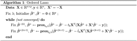
The value γ > 0 is a step size that is adjusted by backtracking to ensure that the objective function is decreased at each step. To solve (3) we augment each predictor x_ij with $x_{ij}^{*}=-x_{ij}$ and write $x_{ij}{\beta }_j=x_{ij}{\beta }_j^{+}+x_{ij}^{*}{\beta }_j^{-}$. We denote the expanded parameters by (β⁺, β⁻) and apply the proximal operator (9) alternatively to X and X* to obtain the minimizers (${\widehat{\beta }}^{+}$, ${\widehat{\beta }}^{-}$). Details for solving (3) can be seen in Algorithm 1. Isotonic regression can be computed in O(N) operations (Grotzinger & Witzgall 1984) and hence Equation (9) can be solved in O(pN) operations. Therefore, the ordered lasso algorithm can be applied to large datasets.

The ordered lasso can be easily adapted to the elastic net (Zou & Hastie 2005) and the adaptive lasso (Zou 2006) by some simple modifications to the proximal operator in Equation (8).

2.3. Comparison between the ordered lasso and the lasso

Figure 1 shows a comparison between the ordered lasso and the standard lasso. The data was generated from a true monotone sequence plus Gaussian noise. The black profiles show the true coefficients, while the gray scale profiles are the estimated coefficients for different values of λ, from largest (at bottom) to smallest (at top). The corresponding plot for the lasso is shown in the bottom panel. The ordered lasso— exploiting the monotonicity— does a much better job of recovering the true coefficients than the lasso, as seen by the fluctuations of the estimated coefficients in the tails of the lasso plot.

Figure 1:

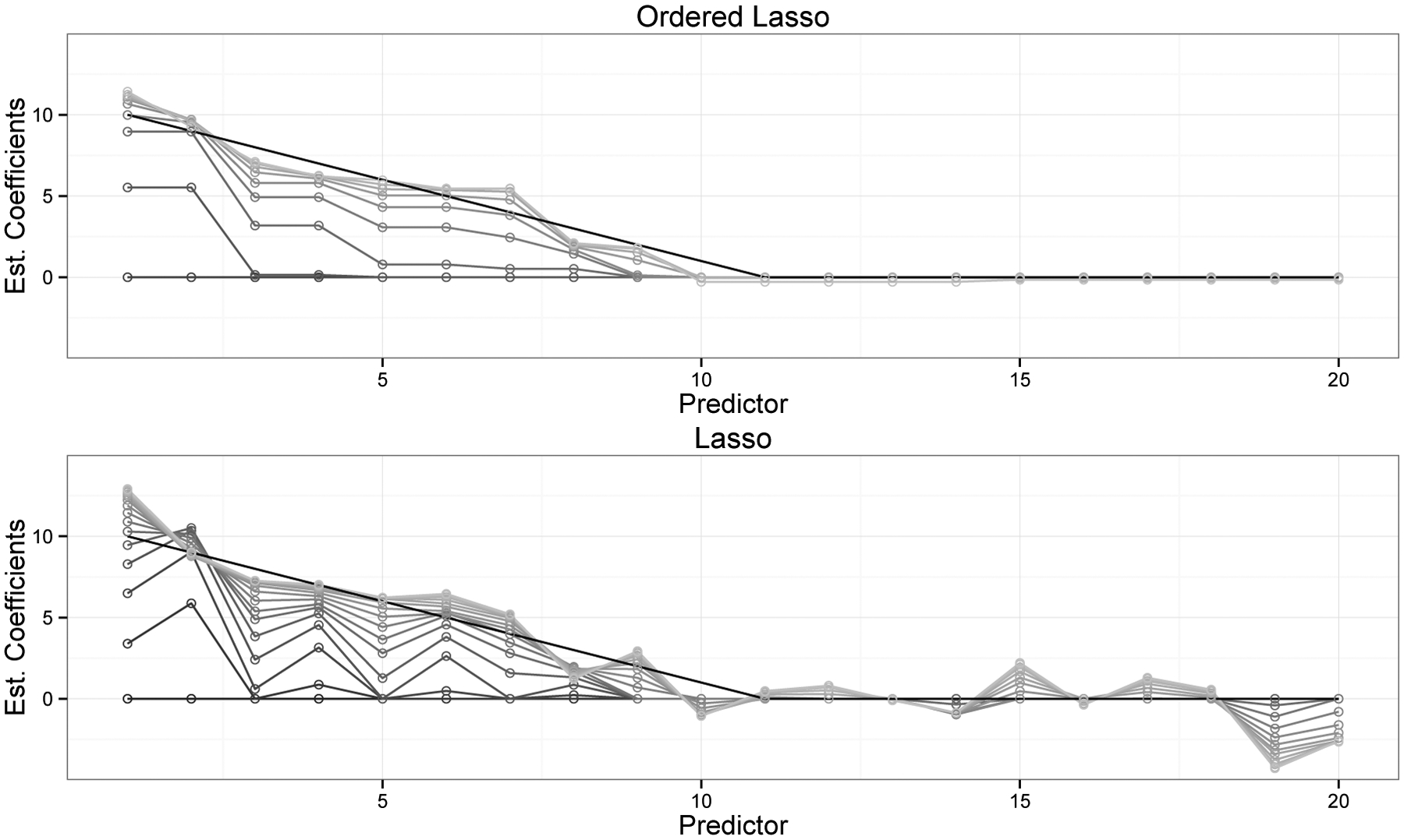
Example of the ordered lasso compared to the standard lasso: the data was generated from a true monotone sequence of coefficients plus Gaussian noise: $y_i={\sum }_{j=1}^p{x}_{ij}{\beta }_j+\sigma \cdot Z_i$, with x_ij ~ N(0, 1), β = (10, 9, …, 2, 1, 0, 0, … 0), σ = 7. There were 20 predictors and 30 observations. The black profiles show the true coefficients and the gray scale profiles are the estimated coefficients for different values of λ from the largest(at bottom) to the smallest(at top).

2.4. The strongly ordered lasso

Previously in the ordered lasso, we wrote ${\beta }_j={\beta }_j^{+}-{\beta }_j^{-}$ and solved for ${\beta }_j^{+}$ and ${\beta }_j^{-}$, for j = 1, 2, ⋯ , p. Though the resulting estimates ${\widehat{\beta }}_j^{+}$ and ${\widehat{\beta }}_j^{-}$ are monotone non-increasing, the resulting solutions ${\widehat{\beta }}_j$ might not be monotone non-increasing in absolute value. To obtain solutions guaranteed to be monotone in absolute value, we extend our procedure: we first compute the minimizers to the ordered lasso problem

$$\underset{{\beta }_0,{\beta }^{+},{\beta }^{-}}{\text{argmin}}\left\{\frac{1}{2}\sum _{i=1}^N{\left(y_i-{\beta }_0-\sum _{j=1}^p{x}_{ij}\left({\beta }_j^{+}-{\beta }_j^{-}\right)\right)}^2+\lambda \sum _{j=1}^p\left({\beta }_j^{+}+{\beta }_j^{-}\right)\right\},$$ (10)

subject to ${\beta }_1^{+}\ge {\beta }_2^{+}\ge \dots \ge {\beta }_p^{+}\ge 0$ and ${\beta }_1^{-}\ge {\beta }_2^{-}\ge \dots \ge {\beta }_p^{-}\ge 0$. Denote solutions to (10) by $\left({\widehat{\beta }}_0,\widehat{\beta }\right)=\left({\widehat{\beta }}_0,{\widehat{\beta }}^{+}-{\widehat{\beta }}^{-}\right)$. Then we let $s\left({\widehat{\beta }}_j\right)$ be the sign of ${\widehat{\beta }}_j$ for j = 1, 2, ⋯ , p and solve

$$\underset{{\theta }_0,\mathit{\theta }}{\text{argmin}}\left\{\frac{1}{2}\sum _{i=1}^N{\left(y_i-{\theta }_0-\sum _{j=1}^p{x}_{ij}{\theta }_j\right)}^2+\lambda \sum _{j=1}^{p}s\left({\widehat{\beta }}_j\right){\theta }_j\right\},$$ (11)

subject to ${\theta }_{1}s\left({\widehat{\beta }}_1\right)\ge {\theta }_{2}s\left({\widehat{\beta }}_2\right)\ge \cdots \ge {\theta }_{p}s\left({\widehat{\beta }}_p\right)\ge 0$. This produces a monotone solution (in absolute value) which is not necessarily the global minimum of the non-convex problem, but is guaranteed to be a stationary point:

Theorem 1. The solution (${\widehat{\theta }}_0$, $\widehat{\theta }$) to (11) exists, and is a stationary point to (2).

The proof of Theorem 1 is presented in the supplementary material.

Compared to the ordered lasso procedure described in Section 2.2, the strongly ordered lasso guarantees the estimated coefficients ${\widehat{\beta }}_j$ monotone non-increasing in absolute value.

2.5. A different relaxation

As suggested by one of the reviewers, we consider the model

$$\underset{{\beta }_0,{\beta }^{+},{\beta }^{-}}{\text{minimize}}\left\{\frac{1}{2}\sum _{i=1}^N{\left(y_i-{\beta }_0-{\sum }_{j=1}^p{x}_{ij}\left({\beta }_j^{+}-{\beta }_j^{-}\right)\right)}^2+\lambda {\sum }_{j=1}^p\left({\beta }_j^{+}+{\beta }_j^{-}\right)\right\},$$ (12)

subject to ${\beta }_1^{+}+{\beta }_1^{-}\ge {\beta }_2^{+}+{\beta }_2^{-}\ge \dots \ge {\beta }_p^{+}+{\beta }_p^{-}\ge 0,{\beta }_j^{+},{\beta }_j^{-}\ge 0$. The constraints in the ordered lasso (3) imply the ordered constraints in (12) but not vice versa. It is also a convex problem and the penalty term encourages sparsity in ${\beta }_j^{+}+{\beta }_j^{-}$ and thus in ${\beta }_j^{+}$, ${\beta }_j^{-}$. The experiments showed that it performs slightly worse than the ordered lasso so we do not consider this formulation further for the rest of paper.

2.6. Relaxation of the monotonicity requirement

As a different generalization of our approach, we can relax problem (3) as follows

$$\underset{{\beta }_0,{\beta }^{+},{\beta }^{-}}{\text{minimize}}\{\frac{1}{2}\sum _{i=1}^N{\left(y_i-{\beta }_0-\sum _{j=1}^p{x}_{ij}\left({\beta }_j^{+}-{\beta }_j^{-}\right)\right)}^2+\lambda \sum _{j=1}^p\left({\beta }_j^{+}+{\beta }_j^{-}\right)+{\theta }_1{\sum }_{j=1}^{p-1}{\left({\beta }_j^{+}-{\beta }_{j+1}^{+}\right)}_{+}+{\theta }_2{\sum }_{j=1}^{p-1}{\left({\beta }_j^{-}-{\beta }_{j+1}^{-}\right)}_{+}\},$$

subject to ${\beta }_j^{+}$, ${\beta }_j^{-}\ge 0$, for j = 1,2 ⋯ , p. As θ₁, θ₂ → ∞, the last two penalty terms force monotonicity in ${\beta }_j^{+}$ and ${\beta }_j^{-}$ and this is equivalent to (3). However, for intermediate positive values of θ₁, θ₂, these penalties encourage near-monotonicity. This idea was proposed in Tibshirani, Hoefling & Tibshirani (2011) for data sequences, generalizing the isotonic regression problem. The authors derive an efficient algorithm NearIso which is a generalization of the well-known PAVA procedure mentioned above. Operationally, this creates no extra complication in our framework: we simply use NearIso in place of PAVA in the generalized gradient algorithm described in Section 2.2.

3. Sparse time-lagged regression

In this section we apply the ordered lasso and the strongly ordered lasso to the time-lagged regression problem. There are two problems we consider. The first one is the static outcome problem, where we observe outcome at a fixed time t and predictors at a series of time points, and the outcome at time t is predicted from the predictors at previous time points. We also consider the rolling prediction problem where we observe both outcome and predictors at a series of time points and the outcome is predicted at each time point from the predictors at previous time points.

3.1. Static prediction from time-lagged features

Here we consider the problem of predicting an outcome at a fixed time point from a set of time-lagged predictors. We assume that our data has the form

$$\left\{y_i,x_{i11},\dots x_{iK1},x_{i12},\dots x_{iK2},\dots x_{i1p},\dots ,x_{iKp}\right\},$$

for i = 1, 2, …, N and N being the number of observations. The value x_ikj is the measurement of predictor j of observation i, at time-lag k from the current time t. In other words, we predict the outcome at time t from p predictors, each measured at K time points preceding the current time t. Our model has the form

$$y_i={\beta }_0+\sum _{j=1}^p\sum _{k=1}^K{x}_{ikj}{\beta }_{kj}+{ϵ}_i,$$

with E(ϵ_i) = 0 and Var(ϵ_i) = σ². We denote ${\widehat{y}}_i={\beta }_0+{\sum }_{j=1}^p{\sum }_{k=1}^K{x}_{ikj}{\beta }_{kj}$, write each ${\beta }_{kj}={\beta }_{kj}^{+}-{\beta }_{kj}^{-}$ and solve

$$\underset{{\beta }_0,{\beta }^{+},{\beta }^{-}}{\text{minimize}}\left\{\frac{1}{2}\sum _{i=1}^N{\left(y_i-{\widehat{y}}_i\right)}^2+\lambda \sum _{j=1}^p\sum _{k=1}^K\left({\beta }_{kj}^{+}+{\beta }_{kj}^{-}\right)\right\},$$ (13)

subject to ${\beta }_{1j}^{+}\ge {\beta }_{2j}^{+}\ge \dots \ge {\beta }_{Kj}^{+}\ge 0$ and ${\beta }_{1j}^{-}\ge {\beta }_{2j}^{-}\ge \dots \ge {\beta }_{Kj}^{-}\ge 0$, ∀j. This model makes the plausible assumption that each predictor has an effect up to K time units away from the current time t, and this effect is monotone non-increasing as we move farther back in time.

In order to solve (13), we first write each ${\beta }_{kj}^{\pm }$ in the following form,

$$\left\{\underset{\text{block }1}{\underbrace{{\beta }_{11}^{\pm },{\beta }_{21}^{\pm },\cdots ,{\beta }_{K1}^{\pm }}}\right|\underset{\text{block }2}{\underbrace{{\beta }_{12}^{\pm },{\beta }_{22}^{\pm },\cdots ,{\beta }_{K2}^{\pm }}}|\cdots \mid \underset{\text{block p}}{\underbrace{{\beta }_{1p}^{\pm },{\beta }_{2p}^{\pm },\cdots ,{\beta }_{Kp}^{\pm }}}\}.$$

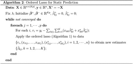
This leads to a blockwise coordinate descent procedure, with one block for each predictor. For example, at step j, we compute the update for block j while holding the rest of the blocks constant. With a sufficiently large time-lag K, the procedure automatically chooses an appropriate number of non-zero coefficients for each predictor, and zeros out the rest in each block because of the order constraint on each predictor. Details can be seen in Algorithm 2.

3.2. Rolling prediction from time-lagged features

Here we assume that our data has the form {y_t, x_t1, …, x_tp}, for t = 1, 2, …, N. In detail, we have a time series for which we observe the outcome and the values of each predictor at N different time points. We consider a time-lagged regression model with a maximum lag of K time points

$$y_t={\beta }_0+\sum _{j=1}^p\sum _{k=1}^K{x}_{t-k,j}{\beta }_{kj}+{ϵ}_t,$$

with E(ϵ_t) = 0 and Var(ϵ_t) = σ². We write each ${\beta }_{kj}={\beta }_{kj}^{+}-{\beta }_{kj}^{-}$ and propose the following problem

$$\underset{{\beta }_0,{\beta }^{+},{\beta }^{-}}{\text{minimize}}\left\{\frac{1}{2}\sum _{t=1}^N{\left(y_t-{\widehat{y}}_t\right)}^2+\lambda \sum _{j=1}^p\sum _{k=1}^K\left({\beta }_{kj}^{+}+{\beta }_{kj}^{-}\right)\right\},$$ (14)

subject to ${\beta }_{1j}^{+}\ge {\beta }_{2j}^{+}\ge \dots \ge {\beta }_{Kj}^{+}\ge 0$ and ${\beta }_{1j}^{-}\ge {\beta }_{2j}^{-}\ge \dots \ge {\beta }_{Kj}^{-}\ge 0$, ∀j. To solve this problem, we convert the problem into the form of Section 3.1. We build a larger feature matrix Z of size N × (Kp), with K columns for each predictor. In detail, each row has the form

$$\left\{x_{t-1,1},x_{t-2,1},\dots ,x_{t-K,1}|x_{t-1,2},x_{t-2,2},\dots ,x_{t-K,2}|\dots |x_{t-1,p},x_{t-2,p},\dots ,x_{t-K,p}\right\}.$$

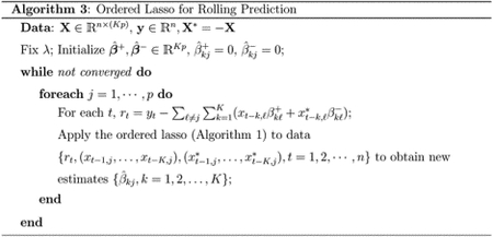
Each block corresponds to a predictor lagged for 1, 2, …, K time units. The matrix Z has N such rows, corresponding to time points t − 1, t − 2, … t − K. Again, we augment each predictor x_t−k,j with $x_{t-k,j}^{*}=-x_{t-k,j}$, choose a sufficiently large time-lag K, and let the procedure to zero out extra coefficients for each predictor. We can solve (14) using block coordinate descent as in the previous subsection. Details are shown in Algorithm 3.

3.3. The strongly ordered lasso applied to time-lagged features

The strongly ordered lasso can be adapted to time-lagged regression by the following two step procedure:

1. Apply Algorithm (2) or Algorithm (3) to obtain signs of the estimated coefficients for each predictor.

2. If there exists a predictor with non-monotone coefficients, apply the strongly ordered lasso procedure to each predictor using blockwise coordinate descent method, as described in Section 3.1.

3.4. Simulated Examples

Figure 2 shows an example of the ordered lasso procedure applied to a rolling time-lagged regression. The simulated data consists of four predictors with a maximum lag of 5 time points and 111 observations. The true coefficients for each of the four predictors were (7, 5, 4, 2, 0), (5, 3, 0, 0, 0), (3, 0, 0, 0, 0) and (0, 0, 0, 0, 0). The features were generated as i.i.d. N(0, 1) with Gaussian noise of a standard deviation equal to 7. The figure shows the true coefficients (black), and estimated coefficients of the ordered lasso (blue) and the standard lasso (orange) from 20 simulations. For each method, the coefficient estimates with the smallest mean squared error (MSE) in each realization are plotted. We see that the ordered lasso does a better job of recovering the true coefficients. The average mean squared errors for the ordered lasso and the lasso were 4.08(.41) and 6.11(.54), respectively.

Figure 2:

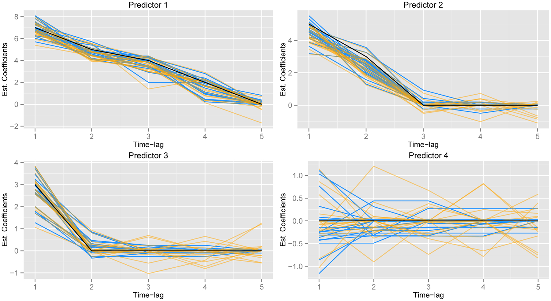
True coefficients (black), coefficient estimates the ordered lasso (blue) and the standard lasso (orange) from 20 simulations.

Figure 3 shows a larger example with a maximum lag of 20 time points. The features were generated as i.i.d. N(0, 1) with Gaussian noise of a standard deviation equal to 7. Let f(a, b, L) denote the equally spaced sequence from a to b of length L. The true coefficients for each of the four predictors were {f(5, 1, 20)}, {f(5, 1, 10),f(0, 0, 10)}, {f(5, 1, 5),f(0, 0, 15)} and {f(0, 0, 20)}. The left panel of the figure shows the mean squared error of the standard lasso and the ordered lasso, over 30 simulations. The value of λ giving the minimum MSE was chosen in each realization. In the right panel we have randomly permuted the true predictor coefficients for each realization, thereby causing the monotonicity to be violated (on average), but keeping the same signal-to-noise ratio. Not surprisingly, the ordered lasso does better when the true coefficients are monotone, while the reverse is true for the lasso. However, we also see that in an absolute sense one can achieve a much lower MSE in the monotone setting of the left panel.

Figure 3:

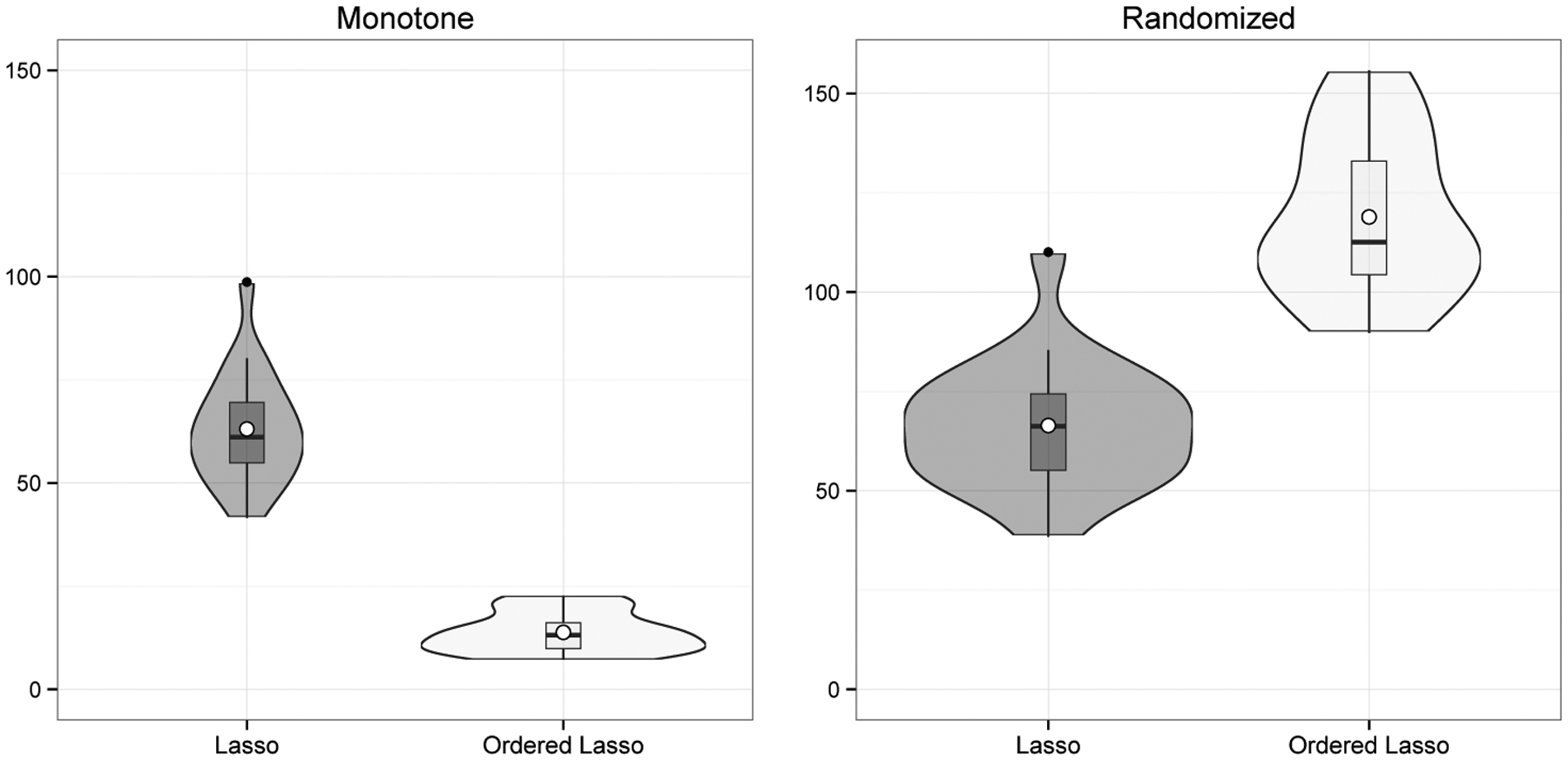
The lasso and the ordered lasso, applied to time-lagged features. Shown is the mean squared error over 30 simulations using the minimizing value of λ for each realization. In the left panel, the true coefficients are monotone; in the right, they have been scrambled so that monotonicity does not hold.

3.5. Performance on the Los Angeles ozone data

These data are available at http://statweb.stanford.edu/~tibs/ElemStatLearn/data.html. They represent the level of atmospheric ozone concentration from eight daily meteorological measurements made in the Los Angeles basin for 330 days in 1976. The response variable is the log of the daily maximum of the hourly-averaged ozone concentrations in Upland, California. We divided the data into training and validation sets of approximately the same size, and considered models with a maximum time-lag of 20 days.

Figure 4 shows the prediction error curves over the validation set, for the “cross-sectional” lasso (predicting from measurements on the same day), the lasso (predicting from measurements on the same day and the previous 19 days), and the ordered lasso, which adds the monotonicity constraint to the lasso procedure. We see that the ordered lasso and the lasso applied to time-lagged features achieve lower errors than the “cross-sectional” lasso. In addition, the ordered lasso achieves the minimum with fewer degrees of freedom (defined in Section 4).

Figure 4:

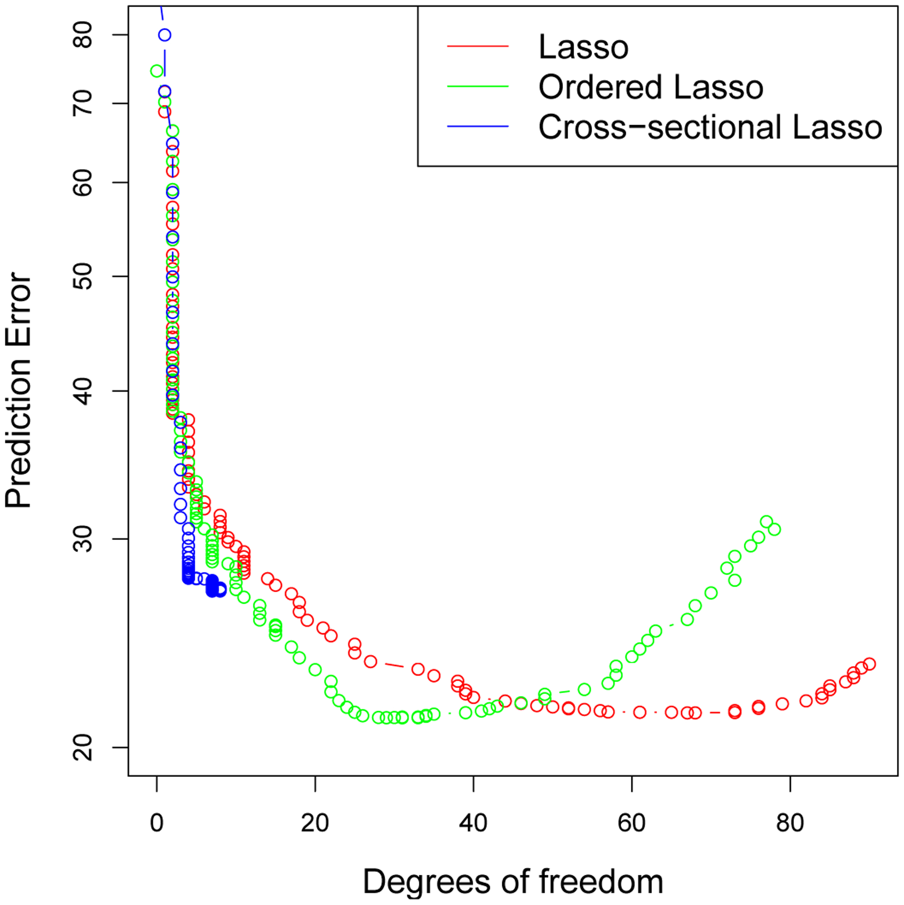
Los Angeles ozone data: prediction error curves. The cross-sectional lasso (blue) predicts from measurements on the same day, the lasso(red) predicts from measurements on the same day and previous 19 days, and the ordered lasso (green) adds the monotonicity constraint to the lasso.

Figure 5 shows the estimated coefficients from the ordered lasso (top), the strongly ordered lasso (middle), and the lasso (bottom). The ordered lasso and the strongly ordered lasso yield simpler and more interpretable solutions. For each predictor, the ordered lasso and the strongly ordered lasso also determine the most suitable estimate of the time-lag interval, beyond which the estimated coefficients are zero. For example, in the ordered lasso plot, the estimated coefficients of the predictor “wind” are zero beyond a time-lag of 14 days from the current time t, whereas the estimated coefficients “humidity” are zero beyond a time-lag of 7 days from the current time t. It is also worth pointing out that even though the ordered lasso yields more interpretable solutions, the estimated coefficients are not monotone non-increasing in absolute value, as marked by blue circles in the top panel of Figure 5. On the other hand, the strongly ordered lasso not only produces a similar plot, but also guarantees the estimated coefficients monotone non-increasing in absolute value.

Figure 5:

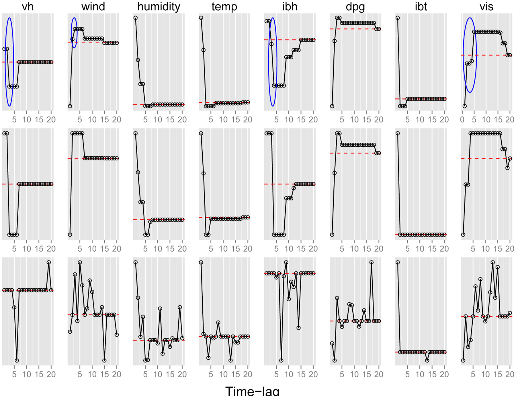
Ozone data: estimated coefficients from the ordered lasso (top), the strongly ordered lasso (middle), and the lasso (bottom) versus time-lag. The blue circles mark regions where the estimated coefficients are not monotone non-increasing in absolute value. For reference, a dashed red horizontal line is drawn at zero.

3.6. Auto-regressive time series applied to sunspot data and simulated data

In an auto-regressive (AR) time series model, one predicts each value y_t from the values y_t−1, y_t−2 … y_t−k for some maximum lag, or “order” k. This fits into the time-lagged regression framework, where the regressors are simply the time series itself at previous time points. Our proposal for monotone constraints in the AR model seems to be novel. Nardi & Rinaldo (2011) studied the application of the standard lasso to the AR model and derived its asymptotic properties. Schmidt & Makalic (2013) suggested a Bayesian approach to the lasso based on the partial autocorrelation representation of AR models. In the following example, we compare coefficient estimates and order estimates among the ordered lasso, the strongly ordered lasso, the lasso, and the standard AR fit.

3.6.1. Performance on the sunspot data

The data for this example is available in the R package as sunspot.year. The data contains 289 measurements and they represent yearly numbers of sunspots from 1700 to 1988. Figure 6 shows the results of the auto-regressive model fit to the yearly sunspot data. We separated the series into training and validation series of about equal size. The standard AR fit (right panel) chose an order of 9 using least squares and the AIC. The ordered lasso (with λ chosen by two-fold cross validation) suggests an order of 10 (out of a maximum of 20) and gives a well-behaved sequence of coefficients. The regular lasso (middle panel) — with no monotonicity constraints— gives a less clear picture. All four estimates had about the same error on the validation set.

Figure 6:

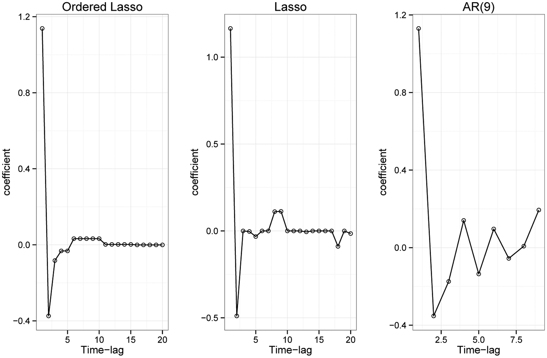
Sunspot data: estimated coefficients of the ordered lasso, the lasso and the standard AR fit.

3.6.2. Performance on simulated data

Table 1 shows the results of an experiment comparing the ordered lasso and the strongly ordered lasso to the standard AR fitting using least squares with AIC and BIC from 100 simulations. The goal was to estimate the lag of the time series (number of non-zero coefficients), as in the previous figure. The true series was of length 1000, with an actual lag of 3, and the maximum lag considered was 10. The data was divided into training and validation series of approximately the same size. The ordered lasso and the strongly ordered lasso used the second half of the series to estimate the best value of λ and estimate the order of the series. The results show that the ordered lasso and the strongly ordered lasso have similar performance to AR/AIC for this task.

Table 1:

Estimates of AR lag from the ordered lasso, the strongly ordered lasso, and AR model using least squares with AIC and BIC from 100 simulations. The data was generated as $y_i={\sum }_{k=1}^3{y}_{i-k}{\beta }_k+\sigma \cdot Z_i$ where σ = 4, y_i, Z_i ~ N(0, 1), and β = {0.35, 0.25, 0.25}. Each entry represents the number of times that a specific lag was estimated in 100 simulations. The results show that the ordered lasso and the strongly ordered lasso have similar performance to AR/AIC for this task.

Method╲Estimated lag	1	2	3	4	5	6	7	8	9	10
AR/AIC	0	0	67	14	7	3	4	3	2	0
AR/BIC	0	0	98	2	0	0	0	0	0	0
Ordered Lasso	0	0	62	16	4	6	4	1	2	5
Strongly Ordered Lasso	0	0	66	14	3	5	3	3	3	3

4. Degrees of freedom

Given a fit vector $\widehat{y}$ for estimation from a vector y ~ N(μ, I · σ²), the degrees of freedom of the fit can be defined as

$$\text{df}(\widehat{y})=\frac{1}{{\sigma }^2}\sum _{i=1}^N\text{Cov}\left(y_i,{\widehat{y}}_i\right)$$ (15)

(Efron 1986). This applies even if $\widehat{y}$ is an adaptively chosen estimate. Zou, Hastie & Tibshirani (2007) show that for the lasso, the number of non-zero coefficients in the solution is an unbiased estimate of the degrees of freedom. Tibshirani & Taylor (2011) give analogous estimates for generalized penalties. For near-isotonic regression described in Section 2.6, letting $\widehat{k}$ denote the number of nonzero “plateaus” in the solution, Tibshirani et al. (2011) show that

$$\text{E}(\widehat{k})=\text{df}(\widehat{y})$$ (16)

For the ordered lasso, this can be applied directly in the orthogonal design case to yield (16). For the general X, we conjecture that the same result holds, and can be established by studying the properties of projection onto the convex constraint set (as detailed in Tibshirani & Taylor (2011)).

Heuristically, one can also perform a significance test to check the monotonicity of the coefficients. We consider testing

$$H_0:{\beta }_1^{+}\ge {\beta }_2^{+}\ge \cdots {\beta }_p^{+}\ge 0;{\beta }_1^{-}\ge {\beta }_2^{-}\ge \cdots {\beta }_p^{-}\ge 0$$

$$H_1:{\beta }^{+}\text{and}{\beta }^{-}\text{not ordered}.$$

We propose the following test statistic and conjecture that it has χ² distribution under the null hypothesis:

$$T=\frac{\left(RSS\left({\widehat{\beta }}_{\text{lasso}}\right)-RSS\left({\widehat{\beta }}_{\text{ordered lasso}}\right)\right)}{{\widehat{\sigma }}^2}~{\chi }_{\text{df}(\text{lasso})-\text{df}(\text{orderedlasso}),}^2$$

where df(orderedlasso) and df(lasso) are defined above.

5. Logistic regression model

Here we show how to generalize the ordered lasso to logistic regression. Assume that we observe (x_i, y_i), i = 1, 2, …, N with x_i = (x_i1, …, x_ip) and y_i = 0 or 1. The log-likelihood function is

$$l\left({\beta }_0,\beta \right)=\sum _{i=1}^N\left(y_i\left({\beta }_0+x_i^T\beta \right)-\text{log}\left(1+e^{{\beta }_0+x_i^T\beta }\right)\right).$$

With the ordered lasso, we write each ${\beta }_j={\beta }_j^{+}-{\beta }_j^{-}$ with ${\beta }_j^{+},{\beta }_j^{-}\ge 0$ for j = 1, 2, …, p and solve

$$\underset{{\beta }_0,{\beta }^{+},{\beta }^{-}}{\text{maximize}}\{l\left({\beta }_0,{\beta }^{+}-{\beta }^{-}\right)-\lambda (\sum _{j=1}^p\left({\beta }_j^{+}+{\beta }_j^{-}\right)\},$$ (17)

subject to ${\beta }_1^{+}\ge \cdots \ge {\beta }_p^{+}\ge 0$ and ${\beta }_1^{-}\ge \cdots \ge {\beta }_p^{-}\ge 0$. We write our data in matrix form and use the iteratively reweighted least squares method (IRLS) to solve (17) (Hastie, Tibshirani & Friedman 2001), i.e., at each iteration we solve

$$\underset{{\beta }_0,{\beta }^{+},{\beta }^{-}}{\text{minimize}}\left\{\frac{1}{2}{\left(z-{\beta }_{0}1-X\left({\beta }^{+}-{\beta }^{-}\right)\right)}^{T}W\left(z-{\beta }_0\mathbf{1}-X\left({\beta }^{+}-{\beta }^{-}\right)\right)+\lambda \sum _{i=1}^p\left({\beta }_i^{+}+{\beta }_i^{-}\right)\right\},$$

subject to ${\beta }_1^{+}\ge \cdots \ge {\beta }_p^{+}\ge 0$ and ${\beta }_1^{-}\ge \cdots \ge {\beta }_p^{-}\ge 0$, where

$$z={\beta }_0^{\text{old}}\mathbf{1}+X\left({\beta }_{\text{old}}^{+}-{\beta }_{\text{old}}^{-}\right)+W^{-1}(y-p),$$

p is a vector with

$$p_i=\frac{\text{exp}\left({\beta }_0^{\text{old}}+x_i^T\left({\beta }_{\text{old}}^{+}-{\beta }_{\text{old}}^{-}\right)\right)}{1+\text{exp}\left({\beta }_0^{\text{old}}+x_i^T\left({\beta }_{\text{old}}^{+}-{\beta }_{\text{old}}^{-}\right)\right)},$$

and W is a diagonal matrix with W_ii = p_i(1 − p_i). We apply the ordered lasso (Algorithm 1) to solve (18) with modified updates:

$${\beta }_0\leftarrow {\beta }_0-\gamma 1^{T}W\left({\beta }_{0}1+X\mathit{\beta }-z\right),$$

$$\beta \leftarrow {\mathbf{\text{prox}}}_{\gamma \lambda }\left(\beta -\gamma X^{T}W\left({\beta }_{0}1+X\mathit{\beta }-z\right)\right).$$

One can also apply the strongly ordered lasso to logistic regression similarly if the estimated coefficients from the ordered lasso are not monotone non-increasing in absolute value.

Applying the ordered lasso to the logistic regression model with time-lagged features, we approximate the log-likelihood function as in (18) and use Algorithm 2 or Algorithm 3 to solve the weighted least squares minimization subproblem. Similar extensions can be made to other generalized linear models.

6. Discussion

In this paper, we have proposed an order-constrained version of the lasso and provided an efficient solution to the resulting problem. This procedure has natural applications to the static and rolling prediction problems, based on time-lagged variables. It can be applied to any dynamic prediction problem, including financial time series and prediction of dynamic patient outcomes based on clinical measurements. For future work, we could generalize our framework to higher dimensional notions of monotonicity, which could be useful for spatial data. The R package orderedLasso that implements the algorithms is available on the CRAN website.

References

- Barlow RE, Bartholomew D, Bremner JM & Brunk HD (1972), Statistical inference under order restrictions; the theory and application of isotonic regression, Wiley, New York. [Google Scholar]
- Bien J, Taylor J & Tibshirani R (2013), ‘A lasso for hierarchical interactions’, Annals of Statistics 42(3), 1111–1141. [DOI] [PMC free article] [PubMed] [Google Scholar]
- Boyd S & Vandenberghe L (2004), Convex Optimization, Cambridge University Press. [Google Scholar]
- de Leeuw J, Hornik K & Mair P (2009), ‘Isotone optimization in R: Pool-adjacent-violators (PAVA) and active set methods’, Journal of Statistical Software 32(5), 1–24. [Google Scholar]
- Efron B (1986), ‘How biased is the apparent error rate of a prediction rule?’, Journal of the American Statistical Association 81, 461–70. [Google Scholar]
- Grotzinger SJ & Witzgall C (1984), ‘Projections onto simplices’, Applied Mathematics and Optimization 12(1), 247–270. [Google Scholar]
- Hastie T, Tibshirani R & Friedman J (2001), The Elements of Statistical Learning; Data Mining, Inference and Prediction, Springer Verlag, New York. [Google Scholar]
- Nardi Y & Rinaldo A (2011), ‘Autoregressive process modeling via the lasso procedure’, Journal of Multivariate Analysis 102(3), 528 – 549. [Google Scholar]
- Schmidt DF & Makalic E (2013), ‘Estimation of stationary autoregressive models with the bayesian lasso’, Journal of Time Series Analysis pp. n/a–n/a. [Google Scholar]
- Shor NZ, Kiwiel KC & Ruszcayǹski A (1985), Minimization Methods for Non-differentiable Functions, Springer-Verlag New York, Inc. [Google Scholar]
- Tibshirani R (1996), ‘Regression shrinkage and selection via the lasso’, Journal of the Royal Statistical Society, Series B 58, 267–288. [Google Scholar]
- Tibshirani R, Hoefling H & Tibshirani R (2011), ‘Nearly-isotonic regression’, Technometrics 53(1), 54–61. [Google Scholar]
- Tibshirani R & Taylor J (2011), ‘On the degrees of freedom of the lasso’, Annals of Statistics (40), 1198–1232. [Google Scholar]
- Wooldridge JM (2009), Introductory Econometrics: A Modern Approach, South-Western College Publishing. [Google Scholar]
- Zou H (2006), ‘The adaptive lasso and its oracle properties’, Journal of the American Statistical Association 101, 1418–1429. [Google Scholar]
- Zou H & Hastie T (2005), ‘Regularization and variable selection via the elastic net’, Journal of the Royal Statistical Society Series B 67(2), 301–320. [Google Scholar]
- Zou H, Hastie T & Tibshirani R (2007), ‘On the “degrees of freedom” of the lasso’, Annals of Statistics 35(5), 2173–2192. [Google Scholar]
Associated Data
This section collects any data citations, data availability statements, or supplementary materials included in this article.