Cryo-Electron Tomography Remote Data Collection and Subtomogram Averaging

Abstract

Cryo-electron tomography (cryo-ET) has been gaining momentum in recent years, especially since the introduction of direct electron detectors, improved automated acquisition strategies, and preparative techniques that expand the possibilities of what the electron microscope can image at high-resolution using cryo-ET and subtomogram averaging software. Additionally, data acquisition has become increasingly streamlined, making it more accessible to many users. The SARS-CoV-2 pandemic has further accelerated remote cryo-electron microscopy (cryo-EM) data collection, especially for single-particle cryo-EM, in many facilities globally, providing uninterrupted user access to state-of-the-art instruments during the pandemic. With the recent advances of Tomo5 (software for 3D electron tomography), remote cryo-ET data collection has become robust and easy to handle from anywhere in the world. This article aims to provide a detailed walk-through, starting from the data collection setup in the tomography software for the process of a (remote) cryo-ET data collection session with detailed troubleshooting. The (remote) data collection protocol is further complemented with the workflow for structure determination at near-atomic resolution by subtomogram averaging with emClarity, using apoferritin as an example.

SUMMARY:

The present protocol describes high-resolution cryo-electron tomography remote data acquisition using Tomo5 and subsequent data processing and subtomogram averaging using emClarity. Apoferritin is used as an example to illustrate detailed step-by-step processes to achieve a cryo-ET structure at 2.86 Å resolution.

INTRODUCTION:

Cryogenic electron microscopy (cryo-EM) is widely known to have experienced a renaissance period accelerating it to become a core and centrally useful tool in structural biology. The development and utilization of direct electron detectors^1–3, improved microscopes and electron sources^3–5, improvements in automation/throughput^6–9, and computational advances in single-particle analysis^10–14 and tomography^15–17 are all in part responsible for the recent success of the technique. These technological drivers have developed cryo-EM’s capability to solve biological macromolecular structures under cryogenic and native conditions. The resolutions that are readily obtainable are sufficient for atomically accurate modeling and have brought the technique to the forefront of the structural biology arena. A reductionist approach in expressing and purifying a biological target of interest has long proven successful in macromolecular crystallography (MX) for basic biological research, drug discovery, and translational science. In the same approach, cryo-EM can now deliver results that parallel high-resolution MX studies. The current major success in the cryo-EM branch of structural biology is called single particle analysis (SPA), which acquires 2-dimensional projection images typically of a purified protein specimen¹⁸ to obtain thousands of views of a biological macromolecule¹⁹. These images contain information from (1) a range of views that fully represent the orientations of the target in 3-dimensional space and (2) capture the object conformational heterogeneity, which can later be separated and investigated.

An alternative approach to acquiring these 2-dimensional projection images of biological samples, even in situ and without purification, is cryo-electron tomography (cryo-ET). Cryo-ET takes a series of images of the same object at tilted angles by mechanically rotating the specimen. Thus the 2-dimensional projections collected in SPA which represent the angular poses of the molecule of interest are collected inherently as part of the cryo-ET imaging experiment²⁰. Tomographic tilt series are then reconstructed into a tomogram which contains 3D representations of the imaged macromolecular complexes. The nature of tomographic data collection does, to a degree, decrease the reliance on averaging to achieve a full 3D representation of a molecule from a collection of 2D images. However, due to current stage designs, the specimen is typically tilted from −60 to +60 °, leaving a missing wedge ²¹ of information in the tomographic 3D reconstruction.

The 3D reconstructions in a single tomogram will then have a missing wedge of information and low signal to noise. To tackle this, individual macromolecules may be extracted as subtomograms and averaged together. Where each macromolecule in a subtomogram is found at a different orientation, the missing wedge will be oriented differently in each subtomogram of the target object, so averaging over many copies will fill in information due to the missing wedge. Recent developments in image processing attempt to train artificial intelligence neural networks to fill in the missing wedge with meaningful data²². This averaging process also increases the signal to noise, akin to the goal of averaging in single particle analysis, so the reconstruction’s quality and resolution improve. If the molecule of interest possesses symmetry, that too may be defined and employed during averaging, further improving reconstruction resolution. The extraction of 3D volumes of a macromolecule from a tomogram into a set of subtomograms and their subsequent processing is known as subtomogram averaging (STA)²³. Where each subtomogram represents a unique copy of the molecule being studied, any structural heterogeneity may be interrogated using the STA workflow. As commonly utilized in the SPA workflow, classification techniques may be employed during STA to dissect the conformational states of the complex of interest. As well as STA enabling high-resolution reconstruction in cryo-ET, this approach makes the technique a powerful tool to interrogate the structural mechanisms of macromolecules in their native cellular environment or of targets often not amenable to SPA^24–26.

Electron tomography has a long history of determining the 3D ultrastructure of cellular specimens at room temperature²⁷. The acquisition of views by physical tilting of the specimen provides enough information for the 3D reconstruction of an object at cellular length scales and is particularly important when cellular structures lack the regularity for averaging. Cells may also be frozen onto substrates for cryo-ET imaging at cell edges where the specimen is thin enough to be electron transparent. Under these conditions, STA may be employed to determine macromolecular structures in a cellular environment, albeit when the specimen is thin enough to be electron transparent²⁸. However, when combined with additional preparative techniques, including cryo-correlative light and electron microscopy (cryo-CLEM) and focused ion beam milling (cryo-FIB), cryo-ET can be used to image inside whole cells under cryogenic conditions²⁹. This brings together the power of cryo-ET to study cellular ultrastructure with the power of STA to determine the structures of macromolecular complexes in situ while identifying their cellular location³⁰ and providing snapshots of complexes engaged in dynamic processes³¹. The ability of the technique to image cellular specimens and employ STA in several studies has highlighted the power of the technique to solve macromolecular structures in situ, even at resolutions comparable to SPA³². A further benefit is found in the knowledge of the original location of the macromolecule represented by the final classified 3D reconstruction in the tomogram³⁰. Therefore, the macromolecular structure can be correlated with cellular ultrastructure. These observations across length scales will presumably lead to important findings where structural mechanisms may be correlated with cellular changes in the context of functional studies.

Cryo-ET and STA allow data collection in three major workflows: molecular, cellular, and lamella tomography. Structures of purified macromolecular complexes may be determined by cryo-ET by molecular tomography. The determination of protein structures in their cellular environment where a cell is thin enough may be described as cellular tomography. More recently, with the development of cryogenic targeting and milling, these same techniques may be applied in lamella tomography workflows to determine protein structures deep inside the cell, in their native environment while revealing the cellular context in which those proteins are observed. Different data collection strategies can be used depending on the available software packages and, most importantly, depending on the requirement of the specimen. Molecular or non-adherent samples on a copper TEM grid of a purified protein typically require less handling and thus remain flat and undamaged in ideal cases. Electron tomograms can easily be set up in series across a holey-carbon grid to quickly acquire tens to hundreds of tomograms in a systematic manner. The simplest way for users to set up molecular tomography samples where proteins are abundantly present on the grid would be to use Tomo5 (software for 3D electron tomography used in the present study, see Table of Materials) Other tomography software such as Leginon and they offer more setup options for more personalized approaches for data collection but are more complex and harder to navigate, particularly for users new to tomography and users accessing their session remotely. For a facility with a large and diverse user base, Tomo5 is easy to operate and train in a remote environment. For adherent cells, grids typically require more handling steps and the necessity to use fragile gold grids increases the need for improved care in handling and data collection strategies. To facilitate finding a cellular region of interest and avoid occlusion from the grid itself at high tilt angles, it is also beneficial to use larger mesh sizes but at the cost that they are inherently more fragile, which can be variable. These factors increase setup time and considerations, but increasing adaptability and robustness again make Tomo5 suitable for this type of data collection. However, specialized data collection scenarios exist for each workflow. BISECT (using SerialEM) introduces the possibility of scripted beam-image shifting during tomography acquisition to increase tomogram collection speed²⁸, particularly in molecular tomography. Medium magnification montages (MM in SerialEM better identify and precisely target molecular features in all workflows. Although, at the time of writing, these features are beginning to be implemented in Tomo5..

Name of Material/Equipment	Company	Catalog Number	Comments/Description
Software
Tomography	Thermo Fisher Scientific	5.9.0	Internal terminology: Tomo5 in document
TEM server	Thermo Fisher Scientific	7.10.1
TIA	Thermo Fisher Scientific	5.10.1
DigitalMicrograph	Gatan	3.44
emClarity	Open-Source software	1.5.3.11	Software for high-resolution cryo-electron tomography and subtomogram averaging
IMOD	Open-Source software	4.11	Modeling, display and image processing programs used for 3D reconstruction and modeling of microscopy images with a special emphasis on electron microscopy data
MotionCor2	Free for academic use	1.1.0	A multi-GPU program that corrects beam-induced sample motion recordedon dose fractionated movie stacks
ETomo	Open-Source software	4.11	ETomo is an interface for running a subset of IMOD and PEET commands.
NoMachine	NoMachine, freeware	7.9.2	Remote desktop software
TeamViewer	TeamViewer AG	-	Remote access and remote control computer software
Materials
Quantifoil (holey support film) EM grids	Quantifoil	-	A flat film of carbon with pre-defined hole size, shape and arrangement
Instrumentation
Titan Krios microscope	Thermo Fisher Scientific	Titan Krios G2
Website
Website 1: https://github.com/bHimes/emClarity/	-	-	Link to download the emClarity software package
Website 2: https://bio3d.colorado.edu/imod/	-	-	Link to download IMOD
Website 3: https://github.com/ffyr2w/emClarity-tutorial	-	-	Link to the emClarity online tutorial
Website 4: https://emcore.ucsf.edu/ucsf-software	-	-	Link to download MotionCor2
Website 5: https://github-wiki-see.page/m/bHimes/emClarity/wiki	-	-	Link to the newest announcements including updates and bug fixs for emClarity

Like SPA, cryo-ET and STA are becoming increasingly accessible through the improvements made to acquisition software and a wealth of available packages for subtomogram averaging^{16,17,32,34–38}. In addition, during the pandemic, enabling remote access to cryo-EM instrumentation became essential to the continued operation of national facilities like the electron Bio-Imaging Centre (eBIC) at Diamond Light Source (DLS), UK. These developments have made cryo-ET more accessible and robust for researchers wishing to utilize the technique. Once data has been acquired, STA is an essential tool for analysing recurrent objects to obtain maximum resolution reconstruction and allow classification of macromolecular heterogeneity. The current protocol aims to provide a detailed walk-through of preparing a cryo-TEM microscope for cryo-ET data collection and how to perform subtomogram averaging using emClarity on a molecular tomography dataset of apoferritin as an example. The use of emClarity (software for high-resolution cryo-electron tomography and subtomogram averaging, see Table of Materials) requires running scripts from the command line, so a level of familiarity with Linux/UNIX systems is assumed.

The remote connection depends on the network environment in each institute/facility. Here, we present a system using programs that allow remote data collection on the specific network configuration used at eBIC, DLS. Remote connection to the microscope is facilitated by two platforms, NoMachine and TeamViewer (see Table of Materials). Using the program NoMachine, the user may log onto a remote Windows desktop. The remote Windows desktop provided by NoMachine resides on the same network as the microscope and thus acts as a virtual support PC to the microscope. From the virtual support PC, the user connects to the microscope via TeamViewer providing direct access and control to the microscope PC running TUI and Tomo.

The present protocol consists of two parts (step 1 and step 2). Step 1 focuses on remote cryo-ET data acquisition using Tomo5 (software for 3D electron tomography). The walk-through for a (remote) session will capture images at increasingly higher magnifications to ultimately allow the user to direct the tomography software to target specimen areas for tomographic data collection. Figure 1 summarizes this process. Step 2 details cryo-ET STA data processing using emClarity (software for high-resolution cryo-electron tomography and subtomogram averaging). The protocol is intended for a remote audience. It assumes the person physically at the microscope and loading the samples has done the direct alignments, taken care of camera tuning, and gain reference acquisition. For this protocol, a 3-condenser lens system with an autoloader is assumed. For further detailed guidelines on the tomography software, a detailed manual by the manufacturer is available in the Windows Start button where the software was loaded from.

Figure 1: Overview of the tomography workflow setup.

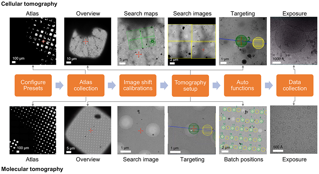
The cryo-ET imaging workflow described in the protocol is shown as a flow chart. The images expected to be acquired are shown for cellular and molecular workflow. The presented naming follows the Tomo5 convention, although most tomography acquisition software share common principles for collecting these images.

PROTOCOL:

1. Remote cryo-ET data acquisition using Tomo5

1.1. If the software is not loaded, begin by starting this software from the TEM server PC (see Table of Materials).

1.2. Perform initial checks and configure the imaging condition by selecting Presets.

1.2.1. Start the session setup by adjusting image acquisition parameters in the Preparation tab under Presets (Figure 2A, B).

Figure 2: Preparation tab and search preset conditions.

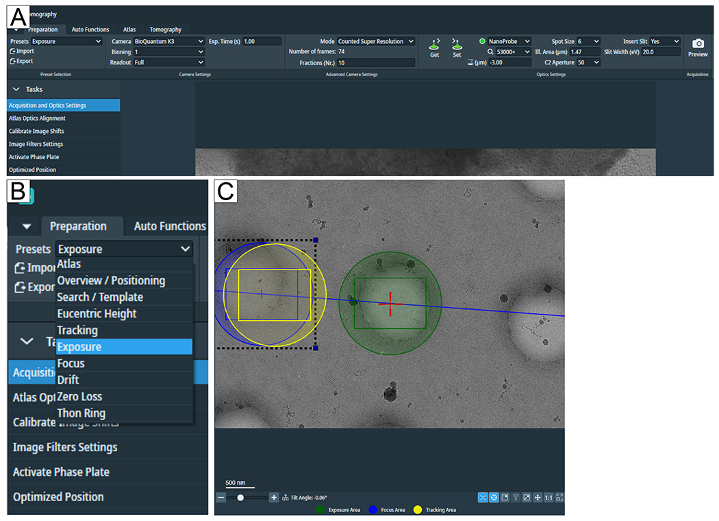
(A) Overview image of the whole tab. Imaging condition presets are set in this tab, and the “Calibrate Image Shift” and “Image Filter Settings” can be found in the “Tasks” flap-out. (B) Zoom in on the “Presets” flap-out where each preset can be selected for individual imaging conditions setup. (C) Image depicting an adequate magnification to fit both the Exposure and the Focus and Tracking area into the field of view.

1.2.1.1. Adjust the “Overview magnification” to suit the grid-square size and dose to get adequate counts.

NOTE: If the suitable magnification is unknown for the grid type, return to this step after loading a grid.

1.2.1.2. “Eucentric Height” and “Search magnification” can be the same. Click on Search in the “Tomography” tab to set up positions and ensure the magnification is adequate to show the feature of interest and to fit both the “Exposure” and the “Tracking/Focus” area in the field of view (Figure 2C).

1.2.1.3. Set “Exposure magnification” to desired target pixel size. If this is unknown, establish it by adjusting the magnification to the desired field of view to fit the region of interest.

1.2.2. Copy the image acquisition (Exposure) parameters to all other high magnification presets (Tracking, Focus, Drift, Zero Loss, Thon Ring). To do so, press Set to set “Exposure” to the microscope and Get to get the “exposure settings” to all other high magnifications after selecting each of them.

1.2.2.1. Adjust exposure times, especially for “Focus” and “Tracking” to give a reasonable number of counts, also taking into account the thickness at 60°, meaning both at 0° and 60°, enough electrons pass through the sample to provide a strong signal for cross-correlation.

NOTE: As an estimate, exposure times for Tracking and Focus equal to the “Exposure” preset are a good first measure. For a dose calculation example for the “Exposure” preset, see Figure 3. Set the calculated exposure time for the “Exposure” preset in the “Preparation” tab.

Figure 3: Dose calculations.

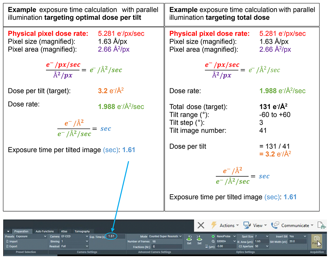
Example dose calculations for possible tomogram acquisition schemes where the dose rate has been measured over vacuum. The two calculations demonstrate determining the exposure time (s) for each tilt, whether targeting an optimal dose per tilt or targeting an optimal total dose for the full tilt series. In subtomogram averaging it is common practice to target an optimal dose per tilted image, in the range of 3.0 – 3.5 e⁻/Ų. In both cases, the Fractions (Nr.) is set to 6 to achieve ~0.5 e⁻/Ų of dose per movie frame of the tilt, for sufficient signal to perform motion correction.

1.2.3. Adjust the “Zero Loss Preset” to use a brighter and larger spot size (larger spot size corresponds to a smaller number; decrease spot size by 2 for K3, and by 1 for Falcon 4), as this needs a higher dose.

NOTE: This preset is best used to align the slit of the energy filter if present on the microscope.

1.3. Perform atlas collection following the steps below.

1.3.1. To collect an atlas, click on the New Session in the “Atlas” tab, set session preferences, enter the storage path and the output format, and press Apply. Select Screening (Figure 4) and then tick all atlases to be acquired. Select Close Col. Valves if you leave the microscope unsupervised this will close the column valves. To start the screening, press the Start button.

Figure 4: Atlas tab.

Overview image of the “Atlas” tab. The image has been cropped to avoid empty grid position spaces. The “Tasks” menu contains session setup preferences and grid selection spaces for individual selection of all grids inventoried and an option to acquire a single atlas after the cassette has been removed from the autoloader. A selected grid can be reset and then re-acquired.

1.3.2. Inspect the single or multiple atlas’ for targets by clicking on the grid in the left panel under “Session Setup” (Figure 4), then left-click and drag the mouse to move around and middle scroll to zoom in-out. Choose grid for target setup, select it and click on Load Sample from inside the software.

1.3.3. For the image shift calibrations, continue to use the atlas screening tab to navigate within the loaded grid. Find an identifiable feature that will be recognizable at all magnification presets, i.e., an ice crystal overlapping with an edge of a hole or another recognizable feature (Figure 5). Move to that square by right mouse click, then Move stage to Grid Square.

Figure 5: Calibrated Image Shifts.

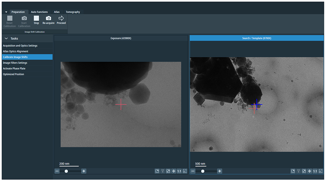
Image depicts an exposure and search image. The red cross in the search image is the shifted marker to correct the offset between exposure and search. Redo image shift calibrations at session start or after changing imaging condition presets.

NOTE: The stage must be at eucentric height to correctly apply image shift calibrations.

1.4. Perform image shift calibration.

1.4.1. In the “Auto Functions” tab (Figure 6), set the preset to “Eucentric Height”, navigate to “Auto-Eucentric” by Stage Tilt, and press Start. Monitor the status window to ensure finding eucentric height is successful and keep an eye on the positive and negative tilt images; they must correlate!

Figure 6: Auto functions and apertures.

(A) The “Auto Functions” tab depicts the “Presets” flab-out and the “Task” selection. Underlined in blue is the “Thon Ring” preset required for “Autostigmate” (also underlined in blue) and “Autocoma”. Select respective presets for each task and then press the Start button. (B) Apertures are found in the TEM User Interface. Select desired “Objective aperture” after the Auto Functions have been performed and run the “Autostigmate” with the aperture in.

NOTE: From version 5.8 of the Tomo software, the criterion for eucentric height acceptance can be modified; the default is within 0.25 μm and setting it to 0.5–0.8 μm gives more leaway. Values depend on microscope performance, but it is recommended to be as small as possible.

1.4.1.1. When at eucentric height and in focus, centre the stage on a feature. Collect a Preview using the “Atlas” preset. Set all “Presets” from the “Preparation” tab. Subsequently, increase the magnification to Overview > centre feature > Preview, then repeat at Search and finally at Exposure magnification.

14.2. If the feature remained centred during targeting, skip the image shift calibrations. Otherwise, to calibrate the image shift, go to the “Preparation” tab, select Calibrate Image Shift, and press Start (Figure 5). This will iteratively align lower magnifications to the feature centred at exposure magnification.

NOTE: The initial preset “Exposure” if centred at this stage; the software will use stage shift for this step only.

1.4.2.1. Press Proceed for the “Exposure” preset. The next image shown will be the “Search preset”. To calibrate the image shift between the presets, double left-click in the Search preview to where the centre of the Exposure preview is, then press Re-acquire (Figure 5). Click on Proceed to move to the next pair of presets.

NOTE: If an image shift at atlas magnification was applied during this calibration, ensure to re-acquire the atlas after the image shift calibration has been completed. Select the desired atlas and press Reset Selected in the top panel in the Atlas tab. Confirm and start acquiring that atlas again.

1.5. Perform the tomography setup.

1.5.1. Create the tomography data collection set up in the “Tomography” tab.

NOTE: Unless specifically stated, the setup is done wholly in the Tomography tab.

1.5.2. Start a New Session. In Session Setup for biological samples, choose Slab-like as sample type and select Batch and Low Dose, select output format and storage folder, optionally add an email recipient, then press Apply.

NOTE: A Batch Positions slab-out now becomes available (Figure 7A). The currently loaded atlas automatically gets imported. “Overview” and “Search images” can be acquired and revisited until a new image is acquired. Additionally, from version 5.8, search maps of 3 x 3, 4 x 4, and 5 x 5 can be acquired with “Acquire Search Map” to ease target finding and setup. They correspond to a version of medium magnification montages.

Figure 7: Tomography tab overview.

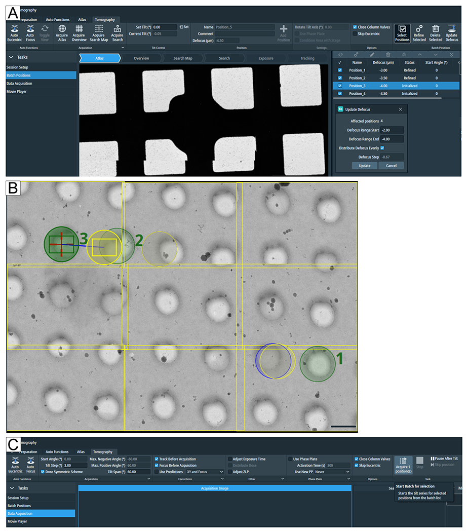
Images show the Tomo 5.8 user interface. (A) Batch Positions. The latest functions depicted in the image: the “Acquire Search Map” option; tomogram positions are shown in atlas view with zoom-in option; highlighted at the top right is “Select Positions”, below all four positions have been selected to “Update Defocus” parameters. (B) Three positions are selected on the search map, labeled 1, 2, and 3. Position 1 will not pose a problem when “Refine All” is run. However, if in a narrow setting such as a lamellae positions are selected as depicted for #2 and #3, then “Refine All” will run the “Tracking” and “Focus” routine on the “Exposure” region of #2, adding dose before the tomogram will be acquired. The grid type is R1.2/1.3. Scale bar = 1.2 μm. (C) Data Acquisition. Selected positions in the Batch Positions flab-out can now be individually acquired.

1.5.3. To set up targets, go to the “Atlas arrow”, find a region of interest and move there by selecting the options that pop up with a right mouse click. Take an Overview image to confirm a good position for eucentric height adjustment, then press on Auto Eucentric; this will run the eucentric by stage tilt routine, then re-acquire a new overview image to update the eucentric height.

NOTE: The “Auto Focus” button should not be necessary if the position is at eucentric height. If the eucentric height image appears far out of focus, the eucentric height is probably not correct and has to be redone (for eucentric height troubleshooting, see Discussion section).

1.5.4. Set the “Overview “ preset before setting up the first position, set the “Overview” preset and tilt the stage to ±60° to check which distance from the grid bars positions can be set up (Figure 8). Perform this by entering the desired tilt angle value into the “Set Tilt” window (Figure 8A).

Figure 8: Defining the maximum tilt angle.

Figures depicted a step-by-step approach to determining the maximum tilt range for tomogram acquisitions. (A) 0 °C overview and a search map in the centre of the grid square. To test the tilt range, the angle can be set in the tomography software with “Set Tilt (°)” by typing the desired value and then pressing Set. (B) The stage has been tilted to −60°, showing that a corner of the search map would not be fully acquired at −60°. (C) The stage has been tilted to 60°. By counting the holes that have disappeared at ±60°, one can get an idea about the tilt range of a grid square. Scale bars = 2.5 μm.

1.5.5. Inspect square Overview or the acquired Search Map, move to a region of interest, and press Acquire Search. Inspect the Search image. If the region of interest is not centered, right-click at the desired position and then repeat Move Stage Here and Acquire Image. Set Tilt (°) to 0.00 (or any other starting angle that the stage can handle) to define starting angle of the tomogram.

1.5.5.1. For the first tomogram, enter the Name for the desired tomogram naming convention and Defocus to set the desired defocus value for each tomogram.

1.5.5.2. Optionally, from Tomo version 5.8 onwards, defocus values can be systematically changed all in one go; for that, click on Select Positions, select positions to be changed, or tick the checkmark to select all positions, then click on Update Defocus and adjust parameters (Figure 7A).

1.5.6. Adjust the “Focus” and “Tracking area” (Figure 2C). Left-click to drag the tracking and focus areas (yellow and blue circles). Ensure the tracking/focus area is (mostly) on carbon or another suitable tracking feature, i.e., a similar feature to the region of interest; avoid cracks, ice contamination, and overly thick regions of empty holes.

1.5.6.1. When choosing blank carbon without many tracking features, ensure that the area starts burning halfway through the tomogram by choosing a high enough dose for focus, and tracking to slowly burn the sample at higher tilts this can be beneficial to keep the tracking accurate. Ensure the tracking/focus area does not expose a later acquisition area.

NOTE: Be aware of what is close and what will come into the beam. Avoid areas with features that will interfere with tracking and/or exposure, including grid bars.

1.5.7. Press Add Position once all parameters are set, and the desired region of interest and “Focus” and “Tracking” are defined. Repeat for new targets.

NOTE: To check the eucentric height is properly calibrated for the batch positions that have been set up, there are several available strategies. Choosing one based on the type of tomography session performed (molecular, cellular, lamella) is recommended.

1.5.8. For molecular tomography, assuming grids are fairly flat, and eucentric height has been done in the centre of each square containing target positions, skip the Refine All (or Refine Selected if positions have been selected, Figure 7A) procedure. If Tomo struggles with the Auto-eucentric by stage tilt routine, possibly click on Skip Eucentric.

1.5.8.1. For cellular or lamella samples, each batch position may be at a different z-height. Either use “Refine All” to be cautious or do not tick the “Skip Eucentric” option.

NOTE: Refine all will iterate through all the tomograms that have been set up or selected via “Select Positions”, refine the eucentric height and check to track and focus before data acquisition. This procedure can expose any overlapping exposure from the next tomogram focus/tracking region (Figure 7B) which should be considered before proceeding.

1.5.8.2. Check and revisit squares that have failed refinement. With the right mouse button, click on the failed position to see options. If eucentric height fails, find “Auto-eucentric” by stage-tilt (step 1.4.1), acquire a new Search image to update the z-height, and Add “Position”. Delete the failed/initialized position. Click on the Skip Eucentric option, which has been done with “Refine all”.

NOTE: If “Refine All” is not run, then “Skip Eucentric” must not be checked as Tomo will run eucentric refinement before each tomogram is acquired; this way, positions that fail eucentric refinement will be skipped.

1.6. Perform Auto functions following the steps below.

1.6.1. Check settings to perform the alignments via the “Auto Functions” tab by navigating in the Atlas to an area of carbon. Bring that area to eucentric height and follow the order of alignments as stated below.

1.6.1.1. Run Auto-eucentric by stage tilt with “Eucentric Height” preset.

1.6.1.2. Run the Autofocus routine with the “Focus” preset.

1.6.1.3. Run the Autostigmate routine with the “Thon Ring” preset.

1.6.1.4. Run the Autocoma routine with the “Thon Ring” preset.

1.6.1.5. Insert the desired Objective aperture (Figure 6B), likely the 100 μm aperture, as a good compromise for increased sample contrast and only a small cut-off in signal at very high resolution.

1.6.1.6. Repeat the Autostigmate routine after aperture insertion.

NOTE: At magnifications with pixel sizes around 3 Å and lower resolutions, the Autocoma routine might fail; in this case, check and align Tomo Rotation Center under the Direct Alignments in the TEM user interface.

1.6.2. Check the Auto Zero-Loss centering routine works on your sample. With the “Zero Loss” preset at a reasonably high dose (step 1.2.3), the routine in Auto Functions will typically succeed over a thin carbon area but can also be done over a vacuum to increase the dose on the detector.

1.7. Perform data collection.

1.7.1. To start the automated acquisition in the Tomography tab, select the Data Acquisition slab-out and set desired parameters (Figure 7C). Set up data acquisition parameters: Tilt Step (°), Max. Positive Angle (°), Max. Negative Angle (°), tracking scheme (recommended: select Track/Focus Before Acquisition). Select Close Column Valves for eucentric height scheme.

NOTE: Rarely used parameters are Adjust Exposure Time, Adjust ZLP, Use Phase Plate, and Pause After Tilt.

1.7.2. Use the “Adjust Exposure Time” for tomograms that are not intended for STA to increase exposure time at a specified ratio at higher tilts.

NOTE: The Adjust ZLP option will run a ZLP refinement after each tomogram, no matter the periodicity set. It is slow and occasionally fails without obvious reasons and will skip that position acquisition. However, it can be useful for very narrow slit width, i.e., 3–5 eV on a Selectris(X) filter.

1.7.3. Phase Plate is used rarely since the introduction of DEDs with energy filters. Ensure that the “Pause After Tilt” does Pause the acquisition but does not allow any changes in the software.

1.7.3.1. Double-check data collection parameters (in the “Preparation” tab), agree with dose calculation and desired tilt scheme, specify the number of Fractions (Nr.) in the “Exposure” preset, then begin acquisition.

NOTE: The number of fractions depends on the sample, the acquisition parameters, and the planned post-processing steps, i.e., STA vs. morphological analysis, and must be kept to values where motion correction and CTF estimation get enough signal. A range of 4–10 fractions is a good estimate, where 4 is more suitable for thicker samples and 10 for thinner molecular samples.

1.7.3.2. Then click on Start to commence data collection and monitor the first tomogram acquisition to ensure tomograms are acquired as intended.

NOTE: Recent tomography software versions have an additional Movie Player slab-out in the Tomography tab where acquired tomograms can be watched. Be patient during the loading process.

2. Cryo-ET STA of apoferritin using emClarity

NOTE: Here, emClarity software¹⁷ is used to illustrate cryo-ET structure determination by STA. Figure 9 summarizes this process. 6 tilts series of apoferritin (EMPIAR-10787) was taken as an example. Octahedral symmetry was applied, and the final map has a resolution of 2.86 Å, obtained from only 4,800 particles and close to the Nyquist frequency (2.68 Å).

Figure 9: emClarity flowchart.

The flowchart described the various steps for cryo sub-tomogram averaging. Scale bars = 50 nm.

2.1. Ensure that the emClarity software package³⁹ is downloaded and installed (see Table of Materials). Install IMOD for the software processing⁴⁰.

NOTE: Basic knowledge of Linux commands is required. A more detailed tutorial can be found in reference⁴¹, which takes a ribosome dataset (EMPIAR-10304) as an example and describes step-by-step procedures. For different types of protein samples, a previously published report is also available⁴².

2.2. Prepare the input files and directories.

NOTE: The raw frames were motion-corrected by MotionCor2 (patch 5 x 5)⁴³. The motion-corrected images were stacked to generate the tilt-series using newstack (IMOD) and manually aligned with patch tracking using Etomo, followed by emClarity. To get better alignments, it is recommended to carry out offsets and tilt compensation in Etomo.

NOTE: The 6 tilt-series are renamed as TS1 to TS6. Below shows the instructions and commands for the first tilt-series (TS1), as an example.

2.2.1. Establish a project folder.

NOTE: The latest version of the software is 1.5.3.11. All the related software logs can be found in the local project folder (…/logFile/emClarity.logfile).

Under the project folder, make another new folder “fixedStacks” and prepare the input files: TS1.fixed, TS1.xf and TS1.tlt. NOTE: TS1.fixed: the original tilt-series, also known as TS1.st in Etomo. TS1.xf: the file contains transformation coordinates after Etomo tiltalign. TS1.tlt: the file contains tilt-angles.

2.3. Estimate the defocus following the steps below.

2.3.1. Calculate the defocus. Update the parameter file with the microscope and imaging parameters following Supplementary Table 1. Copy a parameter file to the project folder, change its name to param_ctf.m and run: emClarity ctf estimate param_ctf.m TS1.

NOTE: The parameter file template can be found in the supplementary information or the local software installation directory (…/emClarity_1.5.3.11/docs/exampleParametersAndRunScript/).

2.4. Check the CTF estimation results for each stack.

2.4.1. Check the aligned stacks (for example, aliStacks/TS1_ali1.fixed) using 3dmod and ensure that the fiducial beads are erased correctly.

2.4.2. Ensure that the handedness is correct, which can be found in logfile/emClarity.logfile.

2.4.3. Check the defocus value (for example, fixedStacks/ctf/TS_ali1_psRadial_1.pdf), and ensure it matches the theoretical CTF estimate.

2.5. Define sub-regions.

2.5.1. Generate a binned tomogram. In the project folder, run: sh recScript2.sh −1.

NOTE: A smaller (in size) tomogram for each stack will be stored in a new folder “bin10”. To speed up the process, the coordinates of one or several sub-regions can be defined in a bin10 tomogram.

NOTE: The script file is in the local software installation directory (…/emClarity_1.5.3.11/docs/).

2.5.2. Determine the boundaries by choosing six points: (xmin, xmax, ymin, ymax, zmin and zmax) to create one sub-region. Under the folder “bin10”, run: 3dmod TS1_bin10.rec.

NOTE: If 4 sub-regions are to be created in one tilt-series, choose 6 × 4 = 24 points. Each stack must have one model file (*.mod) under the folder “bin10”.

2.5.3. Convert the model files to the software format. This will create a new folder recon. Store all the coordinates of each sub-region under this folder. In the project folder, run: sh recScript2.sh TS1.

2.6. Pick particles.

2.6.1. Find an apoferritin template for picking particles. Download a template from Electron Microscopy Data Bank (EMD-10101)⁴⁴. Ensure that the pixel size of the template matches that of the raw data. In the project folder, run: emClarity rescale ApoF.mrc ApoF_Template_rescale.mrc 3.60 1.34 cpu.

2.6.2. Generate CTF-corrected tomograms for particle picking. In the project folder, run: emClarity ctf 3d param_ts.m templateSearch.

2.6.3. Run a particle picking for each sub-region. For the apoferritin dataset, carry out a template search out at bin6. Modify the Tmp_angleSearch parameters [θout, Δout, θin, Δin] to determine the angle range and intervals for in-plane or out-of-plane search in degrees. In the project folder, run: emClarity templateSearch param_ts.m TS1 1 ApoF_Template_rescale.mrc O 1.

NOTE: A folder “convmap_wedge_Type2_bin6” will be generated in this step. The csv file under this folder (for example, TS1_1_bin6.csv) includes all the information about the particles picked.

2.6.4. Remove the incorrect particles using 3dmod. Under the folder “convmap_wedge_Type2_bin6”, run: 3dmod ../cache/TS1_1_bin6.rec TS1_1_bin6.mod.

NOTE: It is common to find wrong particles next to carbon edges or ice contaminations in those areas. Perform right mouse click on the incorrect points and press backspace on the keyboard to delete them. In this step, ensure that most of the false positive points were removed (Figure 10).

Figure 10: Template matching using emClarity.

(A) A typical micrograph of apoferritin on a graphene-coated grid. Defocus: −3.430 μm. (B) A slice of the tomogram overlaid with model points after template searching. (C) A top and (D) a side projection views of model points, indicating a single flat layer of monodispersed apoferritin particles. Scale bars = 50 nm.

2.6.5. Change the folder name “convmap_wedge_Type2_bin6” to “convmap”, as emClarity will go and find sub-region information under convmap in the following steps.

2.7. Initialize the project. In the project folder, run: emClarity init param0.m, to create a database for emClarity, ApoF.mat.

2.8. Perform Tomograms reconstruction before STA and alignment. To generate CTF-corrected sub-region tomograms at bin4, run: emClarity ctf 3d param0.m.

NOTE: CTF-corrected tomograms cache/TS1_1_bin4.rec will be generated in a new folder cache.

2.9. Perform STA and alignment.

2.9.1. Carry out the averaging using the CTF-corrected sub-tomograms starting at bin4. In the project folder, run: emClarity avg param0.m 0 RawAlignment.

2.9.2. Continue to do alignments and run: emClarity alignRaw param0.m 0.

NOTE: The averaging step generates a reference, which will be used by emClarity in this step to align the particles. The Raw_angleSearch parameters [θout, Δout, θin, Δin] can be changed to set the angle range and step sizes for each cycle. As most incorrect particles are removed from the database (Step 2.6.4), these angular settings for alignment can start with a relatively small degree.

2.9.3. Update the Raw_angleSearch parameters and run a few more cycles (Steps 2.9.1 and 2.9.2). To speed up the process, perform in-plane and out-of-plane alignments separately.

NOTE: For each binning, it is recommended to run multiple cycles and gradually reduce the angular settings. For the ApoF dataset, 5 more cycles at bin 4 were carried out and more details can be found in the Supplementary Table 2. For cycle001, in the project folder, run: emClarity avg param1.m 1 RawAlignment, followed by emClarity alignRaw param1.m 1.

2.9.4. Clean the overlapped particles. In the project foler, run: emClarity removeDuplicates param5.m 5.

2.10. Tilt-series refinement with tomoCPR.

NOTE: This step is optional.

2.10.1. Run tomoCPR to refine stack geometry. In the project folder, run: emClarity tomoCPR param5.m 5.

2.10.2. Generate newly aligned stacks and update geometry files. In the project folder, run: emClarity ctf update param6.m.

NOTE: Ensure that the new geometry files (for example fixedStacks/ctf/ TS1_ali2_ctf.tlt) and the newly aligned stacks (for example aliStacks/TS1_ali2.fixed) are correctly generated.

2.10.3. Create new sub-tomograms at bin2. In the project folder, run: emClarity ctf 3d param6.m.

NOTE: This will be followed by a few cycles for averaging and alignment at bin2 (Steps 2.9.1, 2.9.2 and 2.9.3), duplicate cleaning (Step 2.9.4), and optional tomoCPR (Step 2.10). Due to high symmetry, another 5 cycles at bin2 were carried out for apoferritin. Update the Raw_angleSearch parameters for each cycle.

2.11. Perform final reconstruction.

2.11.1. Continue to run a few cycles at bin1 and tomoCPR (Steps 2.9 and 2.10). Another 10 more cycles at bin1 were carried out for the apoferritin dataset. More details regarding the commands and parameters can be found in Supplementary Table 2.

2.11.2. Perform final reconstruction by combining the two half datasets. In the project folder, run: emClarity avg param21.m 21 RawAlignment, followed by emClarity avg param21.m 21 FinalAlignment.

NOTE: The final map (for example with a B-factor of 10, cycle021_ApoF_class0_final_bFact-10.mrc) will be generated, Figure 11.

Figure 11: Cryo-ET STA of apoferritin.

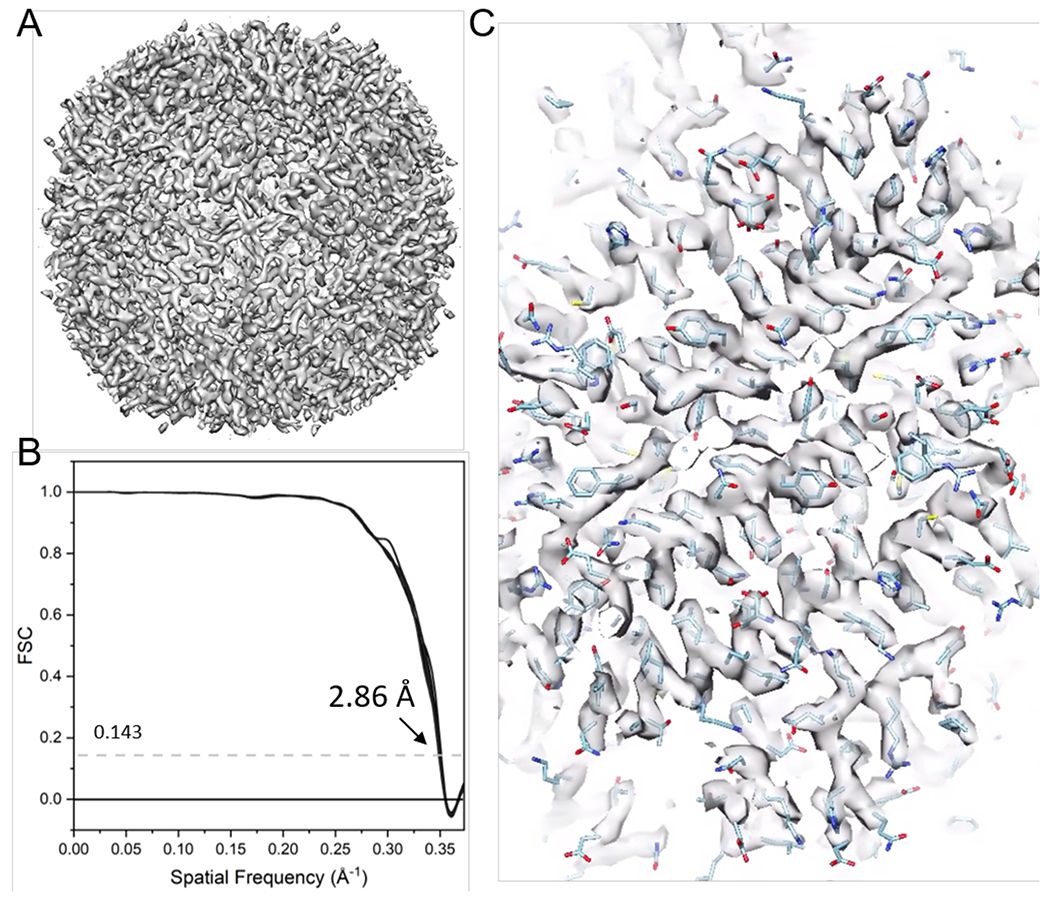
(A) The final map after 21 cycles of sub-tomogram alignment. (B) The final map’s Fourier shell correlation (FSC) plot with a reported resolution of 2.86 Å, containing 38 cone FSCs. (C) Representative density maps (fitted with PDB model 6s61⁴⁶).

REPRESENTATIVE RESULTS:

For cellular and lamella samples, the data collection strategy largely depends on the sample and the goal of the imaging study (Figure 1). The targeting approach will depend on whether the molecular target is in-situ or prepared from the purified macromolecular complex for high-resolution reconstruction specimens containing molecular targets. For purified complexes vitrified onto holey carbon grids, targeting can simply be based on imaging in the holes of the carbon support. For in situ work, the targeting approach requires knowledge of the location of the molecular entity based on correlative data or known low magnification cellular landmarks. Cellular landmarks would ideally be identifiable when taking overview images and, if sufficient to roughly localize regions of interest, can provide a quick way to confirm target identity with a search image. However, if the observable events are rare, then medium magnification search images may be needed to qualify the target is correct. Search maps are medium magnification montages of search images and can thus make target finding much easier, where they can be acquired at a magnification at which the feature of interest is visible. Search maps can then be screened to find and set up target batch positions. For specimens containing cellular features for ultrastructural reconstruction, the targeting approach is similar, though equally dependent on the visibility of the cellular event at various magnifications and its prevalence in the sample.

The data acquisition strategy must also be considered; in all cases, the study’s goal largely determines how the data is collected. For reconstruction of cellular ultrastructure, a low magnification (20–5 Å/px) and large field of view may be appropriate, but high magnifications will be required to reconstruct molecular or high-resolution detail (5–3 Å/px). A dataset collected at 1.5 Å/px under ideal conditions will only physically be able to produce a reconstruction at the Nyquist frequency of 3.0 Å/px; however, in reality, many factors, including but not limited to specimen thickness, size and heterogeneity all affect the obtained reconstruction quality. The exact imaging parameters also balance magnification based on the study’s goal with the field of view to contain enough information. This article presents a subtomogram averaging case reaching 2.86 Å, but additional studies^17,42–45 are presented in Table 1 to illustrate collection parameters associated with studies targeting different outcomes.

Table 1: Collection parameters for several cryo-ET studies.

Studies targeting the reconstruction of molecular detail from purified or in situ proteins compared to a study aiming to resolve and segment ultrastructural cellular features ^17,42,45,47.

Sample	Cryo-ET type	Å/px	Tilt range (+/−)	Tilt step (°)	Defocus range (μm)	Total dose (e−/Å2)	Resolution	Raw data	Reference
Apoferritin	Purified/Molecular (STA)	1.34	60	3	1.5 – 3.5	102	2.86	EMPIAR-10787	17 & this paper
HIV-1 Gag	Purified/Molecular (STA)	1.35	60	3	1.5 – 3.96	120	3.1	EMPIAR-10164	17
Ribosome	Purified/Molecular (STA)	2.1	60	3	2.2 – 4.3	120	7	EMPIAR-10304	42
SARS-CoV-2 spike	Lamella/Molecular (STA)	2.13	54	3	2 – 7	120	16	EMPIAR-10753	45
Neuron axon structure	Cellular (ultrastructural)	5.46	60	2	3.5 – 5	90	N.D.	EMPIAR-10922	47

Once a targeting workflow and data acquisition regime for cryo-ET is established, data collection of many different sample types is possible. Representative tomograms of a variety of specimens are presented here: molecular samples such as apoferritin (Movie 1), thin cellular processes (Movie 2), and FIB milled lamella of the thick cellular specimen (Movie 3).

Movie 1: A tomogram of apoferritin samples on a normal EM grid and then imaged with a Cryo-TEM equipped with a Falcon 4 camera and a Selectris X filter.

Download video file ^{(14.4MB, mp4)}

Tilt series were acquired with a dose-symmetric scheme, with a tilt span of 54° and a total dose of 134 e⁻/A² in the electron tomography software. Scale bar = 50 nm.

Movie 2: A tomogram of a primary neuron grown on an EM grid and then directly imaged with a Cryo-TEM equipped with a Falcon 4 camera and the Selectris filter.

Download video file ^{(16MB, mp4)}

The tilt series were acquired with a dose-symmetric scheme, with a tilt span of 60° and a total dose of 120 e⁻/A² in the electron tomography software. Scale bar = 100 nm.

Movie 3: A tomogram of a Cyanobacteria on an EM grid, subjected to FIB milling and then imaged with a Cryo-TEM equipped with a Gatan K3 camera and a GIB filter.

Download video file ^{(37.4MB, mp4)}

The tilt series were acquired with a dose-symmetric scheme, with a tilt span of 50° and a total dose of 120 e⁻/A² in the electron tomography software. Scale bar = 87.2 nm.

DISCUSSION:

Tomo5

The workflow description of the tomography software highlights one potential and most streamlined way for a (remote) batch tomography session setup. While the software is easy for beginners, some initial cryo-EM experience and basic tomography understanding can help with the setup. Critical steps are highlighted in the protocol and should help troubleshoot even if a different setup approach has been used. The advancement of the software will ease (remote) data collection and make cryo-ET more accessible to a wide user base. A few tips and tricks that can help troubleshoot commonly encountered problems will be described below.

One important point to discuss is the choice of grids because when tilting the specimen to ±60°, i.e., grid bars at high tilts can obscure the view. On a TEM grid the mesh size refers to the number of grid-squares per unit length on the grid. Larger mesh numbers have more grid-squares per unit length, a higher density of grid-squares and so, smaller grid-squares i.e. a 400 mesh grid will have smaller squares than a 200 mesh grid. A good choice of grids for tomography is 200 or 300 mesh grids. As shown in Figure 8, the available area to collect on is reduced as the grid is tilted. At ±60° tilt, a 300 mesh grid will have a smal field of view on which a full tomogram can be acquired. The advantages of 200 mesh grids are that the larger grid-squares make molecular tomography setup faster; and with increased grid-square area, one square will likely be enough for an overnight collection. The disadvantage is that 200 mesh grids are more fragile, so handling and clipping requires more finesse.

Moreover, if using holey support film (see Table of Materials) on EM grids, the hole spacing must be considered for the setup of the focus and tracking region in relation to the exposure region. Ideally, the beam diameter at the desired magnification is small enough to cover the carbon area adjacent to the exposure area along the tilt axis for optimal and fast setup. This way, potential regions of interest in each hole can be acquired on.

As the software’s eucentric height routine is not as robust, such as the serialEM routine, the following tips can work around that problem. If it fails at the eucentric height preset, use the overview preset instead and re-run ‘Auto-eucentric by stage tilt’; this can solve issues if the eucentric height is far away from 0. If this succeeds, re-run ‘Auto-eucentric by stage tilt’ with ‘Eucentric Height’ presets to increase precision. If it fails, run ‘Auto-Eucentric by beam tilt’ with the eucentric height preset and then re-run ‘Auto-Eucentric by stage tilt’ or setup on the square using the z height consolidated by beam tilt. In case grids with a repeating pattern of holes are used, they may prevent the detection of a single cross-correlation peak. Try changing the eucentric height preset to a smaller defocus offset such as −25 μm and/or a shorter exposure time to decrease cross-correlation from hole patterns. On the other hand, using lacey grids or lamella may not be enough signal for a strong cross-correlation peak. Try changing the eucentric height preset to a larger defocus offset such as −75 μm and/or a longer exposure time to improve the cross-correlation peak. Another option is to adjust image filter settings; they can be found in the ‘Preparation’ tab. Options to adjust the filter settings can be set for low (Overview/Gridsquare), medium (Eucentric Height), and high magnification (Tracking/Focus) settings to find the optimal cross-correlation peak for each preset. The required input is one image, i.e., at 0° and one at 5°, followed by clicking Compare to compare both images. Recommended starting values for the longest wavelength are a ¼ of the scale bar in the image and the shortest wavelength to 1/40 of the scale bar. If the peak does not show up nicely, play around with the settings until a convincing peak can be found. There is no need to re-acquire images every time; simply pressing ‘Compare’ is enough. If TOMO still fails to find eucentric height automatically, the manual eucentric height calibration can be used: Centre over a reasonably large ice crystal in overview magnification in the ‘Preparation’ tab, then switch to the ‘Set’ flap out tab in the ‘Stage control’ of the TEM User Interface, set alpha to −30° and adjust z-value to re-centre the crystal using the flu screen image. Selecting ‘High Resolution’ and ‘High Contrast’ settings in the Microscope User Interface will make this easier (buttons at the bottom of the Fluoscreen window). Optionally, if there is access to a camera with live mode, then this can be used to determine the eucentric height; it will be easier than on the fluorescent screen.

From version 5.8 onwards, the most commonly encountered problem for finding the eucentric height, aka an unsuccessful looping around the target z-value, has been solved by implementing the option to set a eucentric height acceptance criterion. However, with different grid and sample types it is highly recommended to adjust the image filter settings to reflect the personal imaging conditions and give the best possible cross-correlation peak to find eucentric height and for the focus and tracking region to stay on track during tomogram acquisition.

The biggest limitations in versions prior to 5.8 have likely been the missing medium magnification montages, the missing dose symmetric scheme, and the problems related to eucentric height finding. These exist in serialEM, a freeware with an outstanding developer and community support, a robust eucentric height routine, and the option to script, i.e., a custom build dose symmetric scheme. However, for facilities that had to switch to remote operation during the pandemic, the software provides an easy access route, and the advancements made in the software will make remote data collections more mainstream in the community.

emClarity

As emClarity uses a template-based particle picking method, it requires a template for the object of interest. The particle picking (step 2.6) is very sensitive and key to the final structure. Before averaging and alignment (Step 2.9), ensure to check carefully and manually remove the false positives. When a template is not available, it might not be easy to use emClarity, but it is possible to use other software, for example, Dynamo³⁷ and PEET⁴⁸, to create an initial model.

For heterogeneous samples, emClarity is equipped with a classification method that enables users to focus on specific features with different scales. It is helpful to run a few cycles of alignments before classification and run it at a higher binning (such as bin 4 or bin 3).

The up-to-date version of the software (V1.5.3.11) has some big updates compared with the first release (V1.0)¹⁷. These include but are not limited to: Handedness check during CTF estimation (Step 2); Symmetry for alignments (CX, I, I2, O); Calculation of per-particle 3D sampling functions (3DSF); Switch to MATLAB 2019a for compatibility and stability; Reconstruction using the raw projection images (cisTEM).

The software will continue to improve for various samples, and the newest announcements can be found online (Please see Table of Materials).

Supplementary Material

Supplementary information

Supplementary Table 1: Data collection and microscope setup details.

Supplementary Table 2. List of commands in the order of execution.

REFERENCES:

- 1.Bai X-C, Fernandez IS, McMullan G & Scheres SHW Ribosome structures to near-atomic resolution from thirty thousand cryo-EM particles. eLife. 2 e00461–e00461, (2013). [DOI] [PMC free article] [PubMed] [Google Scholar]
- 2.Li X et al. Electron counting and beam-induced motion correction enable near-atomic-resolution single-particle cryo-EM. Nature Methods. 10 (6), 584–590, (2013). [DOI] [PMC free article] [PubMed] [Google Scholar]
- 3.Nakane T et al. Single-particle cryo-EM at atomic resolution. Nature. 587 (7832), 152–156, (2020). [DOI] [PMC free article] [PubMed] [Google Scholar]
- 4.Kato T et al. CryoTEM with a Cold Field Emission Gun That Moves Structural Biology into a New Stage. Microscopy and Microanalysis. 25 (S2), 998–999, (2019).31232262 [Google Scholar]
- 5.Yip KM, Fischer N, Paknia E, Chari A & Stark H Atomic-resolution protein structure determination by cryo-EM. Nature. 587 (7832), 157–161, (2020). [DOI] [PubMed] [Google Scholar]
- 6.Mastronarde DN SerialEM: A Program for Automated Tilt Series Acquisition on Tecnai Microscopes Using Prediction of Specimen Position. Microscopy and Microanalysis. 9 (S02), 1182–1183, (2003). [Google Scholar]
- 7.Schorb M, Haberbosch I, Hagen WJH, Schwab Y & Mastronarde DN Software tools for automated transmission electron microscopy. Nature Methods. 16 (6), 471–477, (2019). [DOI] [PMC free article] [PubMed] [Google Scholar]
- 8.Deng Y et al. Smart EPU: SPA Getting Intelligent. Microscopy and Microanalysis. 27 (S1), 454–455, (2021). [Google Scholar]
- 9.Carragher B et al. Leginon: An Automated System for Acquisition of Images from Vitreous Ice Specimens. Journal of Structural Biology. 132 (1), 33–45, (2000). [DOI] [PubMed] [Google Scholar]
- 10.Bell JM, Chen M, Baldwin PR & Ludtke SJ High resolution single particle refinement in EMAN2.1. Methods (San Diego, Calif.). 100 25–34, (2016). [DOI] [PMC free article] [PubMed] [Google Scholar]
- 11.Punjani A, Rubinstein JL, Fleet DJ & Brubaker MA cryoSPARC: algorithms for rapid unsupervised cryo-EM structure determination. Nature Methods. 14 (3), 290–296, (2017). [DOI] [PubMed] [Google Scholar]
- 12.Grant T, Rohou A & Grigorieff N cisTEM, user-friendly software for single-particle image processing. eLife. 7 e35383, (2018). [DOI] [PMC free article] [PubMed] [Google Scholar]
- 13.Zivanov J et al. New tools for automated high-resolution cryo-EM structure determination in RELION-3. eLife. 7, (2018). [DOI] [PMC free article] [PubMed] [Google Scholar]
- 14.Kimanius D, Dong L, Sharov G, Nakane T & Scheres SHW New tools for automated cryo-EM single-particle analysis in RELION-4.0. Biochemical Journal. 478 (24), 4169–4185, (2021). [DOI] [PMC free article] [PubMed] [Google Scholar]
- 15.Galaz-Montoya JG, Flanagan J, Schmid MF & Ludtke SJ Single particle tomography in EMAN2. Journal of Structural Biology. 190 (3), 279–290, (2015). [DOI] [PMC free article] [PubMed] [Google Scholar]
- 16.Bharat TAM & Scheres SHW Resolving macromolecular structures from electron cryo-tomography data using subtomogram averaging in RELION. Nature protocols. 11 (11), 2054–2065, (2016). [DOI] [PMC free article] [PubMed] [Google Scholar]
- 17.Himes BA & Zhang P emClarity: software for high-resolution cryo-electron tomography and subtomogram averaging. Nature Methods. 15 (11), 955–961, (2018). [DOI] [PMC free article] [PubMed] [Google Scholar]
- 18.Weissenberger G, Henderikx RJM & Peters PJ Understanding the invisible hands of sample preparation for cryo-EM. Nature Methods. 18 (5), 463–471, (2021). [DOI] [PubMed] [Google Scholar]
- 19.Au - White JBR et al. Single Particle Cryo-Electron Microscopy: From Sample to Structure. Journal of Visualized Experiments. doi: 10.3791/62415 (171), e62415, (2021). [DOI] [PubMed] [Google Scholar]
- 20.Orlova EV & Saibil HR Structural Analysis of Macromolecular Assemblies by Electron Microscopy. Chemical Reviews. 111 (12), 7710–7748, (2011). [DOI] [PMC free article] [PubMed] [Google Scholar]
- 21.Turk M & Baumeister W The promise and the challenges of cryo-electron tomography. FEBS Lett. 594 (20), 3243–3261, (2020). [DOI] [PubMed] [Google Scholar]
- 22.Liu Y-T et al. Isotropic Reconstruction of Electron Tomograms with Deep Learning. bioRxiv. 10.1101/2021.07.17.452128 2021.2007.2017.452128, (2021). [DOI] [Google Scholar]
- 23.Briggs JAG Structural biology in situ—the potential of subtomogram averaging. Current Opinion in Structural Biology. 23 (2), 261–267, (2013). [DOI] [PubMed] [Google Scholar]
- 24.Grünewald K et al. Three-Dimensional Structure of Herpes Simplex Virus from Cryo-Electron Tomography. Science. 302 (5649), 1396–1398, (2003). [DOI] [PubMed] [Google Scholar]
- 25.Allegretti M et al. In-cell architecture of the nuclear pore and snapshots of its turnover. Nature. 586 (7831), 796–800, (2020). [DOI] [PubMed] [Google Scholar]
- 26.Wang Z et al. The molecular basis for sarcomere organization in vertebrate skeletal muscle. Cell. 184 (8), 2135–2150.e2113, (2021). [DOI] [PMC free article] [PubMed] [Google Scholar]
- 27.Winey M, Meehl JB, O’Toole ET & Giddings TH Jr. Conventional transmission electron microscopy. Molecular biology of the cell. 25 (3), 319–323, (2014). [DOI] [PMC free article] [PubMed] [Google Scholar]
- 28.Davies KM et al. Macromolecular organization of ATP synthase and complex I in whole mitochondria. Proceedings of the National Academy of Sciences. 108 (34), 14121, (2011). [DOI] [PMC free article] [PubMed] [Google Scholar]
- 29.Wagner J, Schaffer M & Fernández-Busnadiego R Cryo-electron tomography-the cell biology that came in from the cold. FEBS Letters. 591 (17), 2520–2533, (2017). [DOI] [PubMed] [Google Scholar]
- 30.Mahamid J et al. Visualizing the molecular sociology at the HeLa cell nuclear periphery. Science. 351 (6276), 969–972, (2016). [DOI] [PubMed] [Google Scholar]
- 31.Erdmann PS et al. In situ cryo-electron tomography reveals gradient organization of ribosome biogenesis in intact nucleoli. Nature Communications. 12 (1), 5364, (2021). [DOI] [PMC free article] [PubMed] [Google Scholar]
- 32.Tegunov D, Xue L, Dienemann C, Cramer P & Mahamid J Multi-particle cryo-EM refinement with M visualizes ribosome-antibiotic complex at 3.5 Å in cells. Nature Methods. 18 (2), 186–193, (2021). [DOI] [PMC free article] [PubMed] [Google Scholar]
- 33.Mastronarde DN Automated electron microscope tomography using robust prediction of specimen movements. Journal of Structural Biology. 152 (1), 36–51, (2005). [DOI] [PubMed] [Google Scholar]
- 34.Kremer JR, Mastronarde DN & McIntosh JR Computer Visualization of Three-Dimensional Image Data Using IMOD. Journal of Structural Biology. 116 (1), 71–76, (1996). [DOI] [PubMed] [Google Scholar]
- 35.Heymann JB & Belnap DM Bsoft: image processing and molecular modeling for electron microscopy. Journal of Structural Biology. 157 (1), 3–18, (2007). [DOI] [PubMed] [Google Scholar]
- 36.Tang G et al. EMAN2: an extensible image processing suite for electron microscopy. Journal of Structural Biology. 157 (1), 38–46, (2007). [DOI] [PubMed] [Google Scholar]
- 37.Castaño-Díez D, Kudryashev M, Arheit M & Stahlberg H Dynamo: A flexible, user-friendly development tool for subtomogram averaging of cryo-EM data in high-performance computing environments. Journal of Structural Biology. 178 (2), 139–151, (2012). [DOI] [PubMed] [Google Scholar]
- 38.Hrabe T et al. PyTom: A python-based toolbox for localization of macromolecules in cryo-electron tomograms and subtomogram analysis. Journal of Structural Biology. 178 (2), 177–188, (2012). [DOI] [PubMed] [Google Scholar]
- 39.Himes BA GitHub: emClarity. (2021). [Google Scholar]
- 40.Mastronarde DN The IMOD Home Page, <https://bio3d.colorado.edu/imod/> (2020). [Google Scholar]
- 41.Frosio T GitHub: emClarity-tutorial, <https://github.com/ffyr2w/emClarity-tutorial> (2021). [Google Scholar]
- 42.Ni T et al. High-resolution in situ structure determination by cryo-electron tomography and subtomogram averaging using emClarity. Nature protocols. 17 (2), 421–444, (2022). [DOI] [PMC free article] [PubMed] [Google Scholar]
- 43.Zheng Palovcak, Armache Cheng & Agard. MotionCor2, <https://emcore.ucsf.edu/ucsf-software> (2016).
- 44.Mills DJ, Pfeil-Gardiner O & Vonck J Apoferritin from mouse at 1.84 angstrom resolution, <https://www.emdataresource.org/EMD-10101> (
- 45.Nedozralova H et al. In situ cryo-electron tomography reveals local cellular machineries for axon branch development. Journal of Cell Biology. 221 (4), e202106086, (2022). [DOI] [PMC free article] [PubMed] [Google Scholar]
- 46.Vonck J, Pfeil-Gardiner O & Mills DJ Apoferritin from mouse at 1.84 angstrom resolution, <https://www.rcsb.org/structure/6s61> (2019).
- 47.Mendonça L et al. Correlative multi-scale cryo-imaging unveils SARS-CoV-2 assembly and egress. Nature Communications. 12 (1), 4629, (2021). [DOI] [PMC free article] [PubMed] [Google Scholar]
- 48.Nicastro D et al. The molecular architecture of axonemes revealed by cryoelectron tomography. Science. 313 (5789), 944–948, (2006). [DOI] [PubMed] [Google Scholar]
Associated Data
This section collects any data citations, data availability statements, or supplementary materials included in this article.
Supplementary Materials