The Use of Extreme Value Statistics to Characterize Blood Glucose Curves and Patient Level Risk Assessment of Patients With Type I Diabetes

Abstract

Objective:

Characterizing blood glucose curves and providing precise patient level risk assessment of hyperglycemia using extreme value statistics and comparing these assessments with traditional indicators of glycemic variability which are not designed to specifically capture the risk of hyperglycemia.

Research Design and Methods:

One year return level (blood glucose level exceeded exactly once every year on average) and probability of exceeding and expected time spent above certain thresholds (600 and 400 mg/dL) per year were calculated. As a comparison, traditional metrics for glycemic variability were determined too. The effect of body mass index on extremes was also investigated using non-stationary models. Metrics were calculated on a dataset containing 170.8 patient-years of measurements of 226 patients.

Results:

Nine high-risk patients were identified with the novel metrics: their estimated time spent above 600 mg/dL per year were above 2 hours. These patients were at moderate risk according to the traditional metrics. Higher body mass index was associated with more extreme glucose levels.

Conclusions:

Through these estimates it is possible to assess each patient’s individual clinical risk of hyperglycemia even beyond the observed blood glucose levels and detection limits. Additionally, it allows the assessment of the impact of clinical characteristics and treatments on blood glucose control in a novel, mathematically well-founded and potentially clinically more useful way than the already existing indicators.

Introduction

Extreme value statistics (EVS) is a branch of statistics investigating the distributions of observations with unusually low or high values, thus it finds natural applications in biomedical science. ¹ Despite that, few examples exist for such approaches in medicine, in contrast to fields like architecture, ² weather and climate analysis, ³ sports, and finance statistics,^4,5 where rare, extreme events have an overwhelming impact too. Because of the rarity of these events or observations, they form just a fraction of the total sample, thus have much smaller effective sample size, therefore their analysis could be exceptionally difficult. EVS is rarely used in medical statistics, the main reason being the lack of data on extremes and the cost of obtaining them compared to natural factors like weather which is simple and cheap to observe and abundant data are publicly available, with daily or even higher frequency and recorded for decades. In contrast, even for very severe conditions, important biomarkers are usually those that require some sample taken which is typically followed by a complex and expensive process to analyze that; thus, it might be measured for patient maybe a couple or dozen times through their clinical history and that is often enough for clinical decision making.

However, advances in measurement technology make diabetology an exception. In particular, with the widespread availability of continuous glucose monitoring (CGM), high-frequency (typically 5 minutes sampling time) and longer-term (up to a week even in routine clinical practice) measurements became possible relatively long time ago. ⁶ But metrics to measure glycemic variability (GV) from blood glucose curves provided by CGM are still not optimal and widely agreed upon^7-9 even until very recently. ¹⁰ Additionally, the lack of accuracy and reliability limits their use in clinical practice. ¹¹ Even more importantly, while GV and risk of hyperglycemia are likely correlated, traditional GV metrics are inherently limited as hyperglycemia risk metrics as they are very insensitive to high values if there are only a few of them. This is in contrast both to intuition (even a single or very few measurements above, say, 400 mg/dL raises the fear that the patient has a high risk of hyperglycemia) and to the mathematical behavior of extreme values as described by EVS.

The current practice of summarizing continuously measured blood glucose curves uses several indicators, such as the Mean Amplitude of Glycemic Excursions (MAGE), ¹² using glycemic excursions in excess of 1 standard deviation (SD) above the mean, the Continuous Net Overall Glycemic Action (CONGA), ¹³ which is the SD of the differences between measurements taken at regular time intervals, simple coefficient of variation (CV; ratio of the SD to the mean), interquartile range, or percentage time spent in, above or below standardized clinical target glucose ranges ¹⁴ or the control-variability grid analysis (CVGA) plot ¹⁵ (which is essentially the same, but in graphical form) and other type of graphical tools ¹⁶ and composite metrics ¹⁷ which enable the rapid evaluation of the CGM measurements collected for several days or weeks.

Instead of these metrics, EVS allows the estimation of the probability that the measurement exceeds a certain threshold (which is the relevant factor for hyperglycemia), even if such values were never observed in the sample. By taking the sampling frequency into account, this can be used to calculate the probability that the patient’s blood glucose will be above a threshold in a given time span (e.g., in 1 year) and the expected time spent above the threshold in the interval. The concept of return level is also often used in EVS: this is the level, blood glucose value in the present case, that is expected to be exceeded exactly once in every year (or any other time interval specified, usually called the return period).

Taken together, these factors raise the possibility that metrics based on EVS are more useful to accurately capture the risk of hyperglycemia.

Following our previous works^18,19 the aim of the present study is therefore the investigation of how EVS can be applied to characterize blood glucose curves and provide patient level risk assessment of hyperglycemia.

Methods

Blood glucose measurements will be considered as realizations of a random variable, that is, instead of analyzing it on the time domain, we will focus on the extremes of these observations; for simplicity, the modeling of maximum will be considered here.

The behavior of the maximum of random variables were described by Ronald Fisher and Leonard Henry Caleb Tippett in 1928 ²⁰ and this result was later proven by Boris Vladimirovich Gnedenko in 1943. ²¹ Together these form the Fisher–Tippett–Gnedenko theorem which establishes that if there are constants with which the maximum of independent and identically distributed random variables can be linearly transformed so that this renormalized variable converges to a non-degenerate distribution, then this distribution must be one of the following:

$$F\left(x\right)=\exp \left[-{\left\{1+\xi \left(\frac{x-\mu }{\sigma }\right)\right\}}_{+}^{-\frac{1}{\xi }}\right]if\xi \ne 0$$

$$F\left(x\right)=\exp \left[-\exp \left\{-\left(\frac{x-\mu }{\sigma }\right)\right\}\right]if\xi =0$$

Here $\mu \in R$ is the location, $\sigma >0$ is the scale and $\xi \in R$ is the shape parameter.

While this formulation is suitable for analysis from the probability theory point of view, in statistical investigation the maxima has to be estimated. A sample is needed, so we can’t simply take the maximum of the whole series. One of the possible solutions is the so-called block maxima (BM) method, which first splits the data to equal sized blocks and takes only the maximum of each block to form a secondary sample to analyze, that is, BM are used to capture maxima.

It should be noted that blood glucose observations are temporally dependent (likely positively autocorrelated). Fortunately, this causes minimal difficulty in case of the BM approach (in contrast to the other, so-called peak over threshold approach). ²² In the BM method, local dependence is much less of concern, and even for the long-term dependence only a rather weak condition (the so-called D(u_n) condition of Leadbetter) ²³ is required to ensure that BM of the dependent data will have the same distribution as independent data would have. It is true that the parameters will be different if the data are dependent, but as parameters are estimated from the sample anyway, it causes no problem. ²² (The drawback of the BM approach is the less efficient use of sample size, but as we now have very large samples this is of less concern.)

Patient Data

The REPLACE-BG ²⁴ trial’s dataset excluding the calibration measurements obtained through the T1D Exchange ²⁵ was used in the present investigation containing 14.8 million CGMS measurements of 226 patients (median duration: 33 weeks) with Type I diabetes. The sampling frequency was 5 minutes using Dexcom G4 Platinum CGM device (Dexcom, San Diego, California). Basic clinical data (except age) were available for all patients.

The patients were relatively homogeneous due to the inclusion and exclusion criteria of the REPLACE-BG study. ²⁴ Of note, patients with more than 1 episode of diabetic ketoacidosis (DKA) in the past year were excluded, and it is also known that no patient had DKA during the study. Patients with an estimated glomerular filtration rate <30/min/1.73 m² obtained within the prior 12 months as part of usual care or kidney transplant were excluded as well, and no serious events occurred that could have realistically led to renal dialysis or mannitol administration. ²⁴ Seven participants were hospitalized for a total of 8 times, including a single surgery; none of these were related to glucose metabolism. ²⁴

Patients were on insulin pump for at least 3 months prior to the starting of the measurements and were not using a low-glucose-suspend function. ²⁴ We had no information on the actual pump usage, but due to the inclusion criteria of REPLACE-BG it could be assumed that no long-term lack of pump usage occurred during the measurements.

Classical Metrics

Classical metrics were calculated for each patient. These metrics included the time spent in standardized ranges specified by Battelino et al, ¹⁴ mean daily CONGA, ¹³ CV, ²⁶ interquartile range (IQR), ²⁷ and mean daily MAGE ¹² and MAGE+ which is the same but for the ascending phases only.

Statistical Methods

Block maxima method was used to analyze the dataset. Two different models were investigated: one in which each parameter is allowed to be different from patient to patient, and a non-stationary in which all parameters were allowed to be—linear—functions of BMI.

Probabilities for exceeding, and estimated time spent above the clinically relevant level of 600 mg/dL (threshold for diabetic hyperosmolar syndrome) ²⁸ and 400 mg/dL, in addition to 1 year return level were calculated for each patient. Neither missing clinical nor CGM data were imputed.

Programs Used

The analysis was carried out using the R statistical program package version 4.1.0 ²⁹ with ExtRemes 2.1 ³⁰ and gluvarpro 4.0 ³¹ packages.

Results

Patient Characteristics

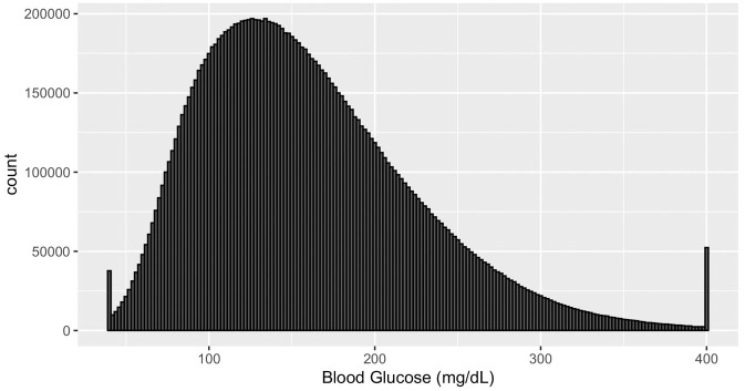
The histogram of all measurements are shown in Figure 1. We can observe a skewed distribution with 2 “spikes” at the two ends of the histogram which strongly indicates that there are lower and upper detection limits present leading to the loss of information. Dexcom G4 Platinum’s user’s manual ³² confirms that the detection limits are 40 to 400 mg/dL. We found no literature that investigates the impact of the presence of an upper detection limit on GV metrics.

Figure 1.

Histogram of all CGM measurements. Abbreviation: CGM, continuous glucose monitoring.

Of the 226 patients, 114 (50.5%) were male, mean age was 44 years (SD = 14) and mean HbA1c was 7.0 (SD = 0.6) at baseline, however due to the anonymization, only height, weight and ethnicity were available on patient level.

Risk Assessment of Hyperglycemia of Individual Patients

The BM models were fitted to the dataset with the block maximum calculated with a block size of 12 (of 5 minutes long periods, i.e., hourly maxima were calculated) for each patient’s CGM record separately so all 3 parameters of the generalized extreme value distribution were estimated individually.

The median and (range) of the parameters were: shape $\widehat{\xi }:-0.077$ (-0.432, 0.107); location $\widehat{\mu }:150.2$ (94.6, 251.5) and scale $\widehat{\sigma }:52.3$ (15.4, 100.3). The distribution of the parameters of the fitted models for each patient can be found in Figure S1.

Results expressed as return levels with their 95% confidence interval (CI) are plotted in Figure S2; CIs indicate reasonably precise estimates.

With the BM approach we were also able to calculate the probability that the blood glucose level exceeds a certain threshold, as the appropriate quantile of the fitted distribution and through this we are able to estimate the proportion or actual time spent above this threshold.

The expected number of hours spent above 600 mg/dL (Figure S3) and above 400 mg/dL (Figure S4) over a year were also plotted.

Comparison with Classical Metrics

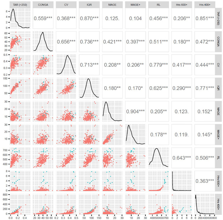
The distribution and relationship of classical GV metrics and the metrics calculated with EVS (1 year return level and hours spent above 600 and 400 mg/dL) are shown on Figure 2 and Figure S5. The highlighted patients are those 9 patients who are estimated to spend more than 2 hours above 600 mg/dL a year, thus are at highest risk of hyperglycemia. Figure 2 shows that these patients had moderate scores in percentage time above range (TAR) >250 mg/dL, CONGA, IQR and MAGE but were in the top third in Coefficient of Variation and—obviously—had the highest return levels. It also shows that they had the their estimated times above 400 mg/dL is mixed: a patient can spend more time above 400 mg/dL but less above 600 mg/dL or the other way around and the low correlation between these too metrics is due to that the majority of their values were zero.

Figure 2.

Pairwise scatterplots, distribution and linear correlation coefficients of the investigated metrics. Distribution of each metric can be found in the main diagonal, pairwise correlation coefficients in the upper right triangle and their pairwise scatterplots in the bottom left half. The 9 highest risk patients according to the estimated time above 600 mg/dl obtained with EVS are highlighted. Abbreviations: CONGA, continuous net overall glycemic action; CV, coefficient of variation; EVS, extreme value statistics; Hrs 400+, EVS estimation of hours spent above 400 mg/dl per year; Hrs 600+, EVS estimation of hours spent above 600 mg/dl per year; IQR, interquartile range; MAGE, mean amplitude of glycemic excursions; RL, return level; TAR (>250), observed time above range (TAR) spent above >250 mg/dl.

Return level and hours spent above 400 mg/dL were compared with standardized clinical ranges ¹⁴ in Figure S5 with the same patients highlighted as in Figure 2. Interestingly, the estimated time spent above 400 mg/dL had a strong negative correlation with the time in (target) range (TIR 70-180) and as expected correlated with the categories corresponding to the higher glucose levels similarly to the return level.

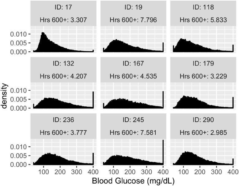
The histogram of CGM measurements of the 9 high risk patients show that 8 of them were heavily affected by the detection limits (Figure 3). Looking at the top 20 patients (Figure S6) the ratio of patients relevantly reaching the upper detection limit is still very high.

Figure 3.

Histograms of CGM measurements of the patients with the highest risk. Abbreviation: CGM, continuous glucose monitoring.

Non-Stationary Models: The Impact of BMI

Additionally, we modeled the effect of BMI on blood glucose extremes using a non-stationary model where all 3 parameters might depend on BMI. The effect of BMI on all parameters was statistically significant, with each unit of BMI changing the shape parameter with ${\widehat{\beta }}_{{\xi }_1}=-0.0025$ (95% CI: -0.0028, -0.0022), the location parameter with ${\widehat{\beta }}_{{\mu }_1}=0.76$ (95% CI: 0.73, 0.79), and the scale parameter with ${\widehat{\beta }}_{{\sigma }_1}=0.400$ (95% CI: 0.381, 0.418).

The overall effect of BMI on the distribution of the hourly maximum is shown in Figure 4. Compared to the reference level of 20, having 40 BMI was associated with a flatter distribution thus higher variability and a shift toward higher values and prolonged tail. Note that despite BMI added as a linear parameter its effect on the results is non-linear, as maxima depends non linearly on the shape parameter.

Figure 4.

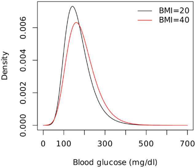
The effect of BMI on the distribution of the hourly maximum blood glucose. Abbreviation: BMI, Body Mass Index.

Accuracy of CGM Measurements

The validation of CGM measurements, especially unusual values was essential; fortunately, the REPLACE-BG dataset included confirmatory blood glucose measurements (BGM).

We compared CGM measurements over 300 mg/dL with corresponding blood glucose measurements within +/- 2.5 minutes time frame where this was available (N = 15,965). These were plotted against each other and assessed graphically (Figure S7).

Additionally, Figure S8 shows the histogram of the corresponding blood glucose measurements where the CGM measurement was exactly 400 mg/dL (N = 1,603).

These analyses show that BGM values randomly scatter around CGM values, and, importantly, this is true even for the case when CGM was 400 mg/dL. Should those CGM measurements result from a malfunction (which won’t affect the BGM), the results wouldn’t scatter around the CGM value, thus this finding rules out the possibility of a systematic error with high certainty.

Discussion

Previously in the biomedical field, EVS methods like the BM approach were rarely used. Although EVS was used to analyze cholesterol levels ³³ or pneumonia and influenza deaths, ³⁴ the lack of sufficient data is a serious limitation in the application of EVS in biomedical field. Our study is the first where EVS was applied in diabetology, moreover on a particularly large dataset.

Our aim was to demonstrate that EVS enables us to characterize a blood glucose curve focusing on the more relevant extremes if hyperglycemia risk is to be captured, which can be used—among others—to create patient-level summary metrics and to assess the impact of clinical characteristics or treatments in a more precise and practical way.

In general there are not many patients who got high score according to the classical metrics but low score with the EVS metrics, but for EVS-based metrics, the patients with the highest values (and thus the highest attributable risk) had moderate values with the regular metrics meaning they were not identified as high-risk patients using regular values. The examination of these cases shows that these patients often reached the upper detection limit of the CGMS sensor at 400 mg/dL.

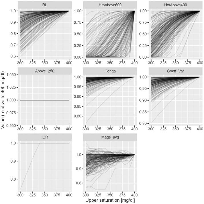
Our hypothesis was that traditional GV metrics are inherently limited as hyperglycaemia risk metrics as they are insensitive to high values if there are only a few of them. To investigate this issue, we performed an additional analysis: we checked the behavior of both traditional variability metrics and our new, proposed metrics if saturation point is artificially lowered by replacing values above it with the saturation point. This essentially means testing on a synthetic dataset, i.e., we could simulate the effect of saturation this way (of course only for saturation levels < 400 mg/dL). Results shown on Figure 5 and Figure S9 confirmed that traditional metrics are very insensitive to saturation (i.e., extreme values) making them unlikely to be a good metric for the risk of hyperglycemia, in contrast to our proposed metrics.

Figure 5.

Impact of upper saturation level (trimming) on traditional GV metrics and metrics based on EVS. Values obtained with the given upper saturation level were divided with the original value (i.e., when only the physical 400 mg/dl saturation level was in effect). Abbreviations: CONGA, continuous net overall glycemic action; CV, coefficient of variation; EVS, extreme value statistics; GV, glycemic variability; Hrs 400+, EVS estimation of hours spent above 400 mg/dl per year; Hrs 600+, EVS estimation of hours spent above 600 mg/dl per year; IQR, interquartile range; MAGE, mean amplitude of glycemic excursions; RL, return level; TAR (>250), observed time above range (TAR) spent above >250 mg/dl.

Through the non-stationary analysis we found that higher BMI is associated with higher variability. This is in contrast to a previous study, that reported an association of higher BMI with lower glycemic variability metrics. ³⁵

The assessment of the confirmatory blood glucose measurement was based upon a large sample and characterized the level and distribution of measurement errors at high glucose levels and the findings confirmed that our results were based on valid measurements.

Conclusion

The main advantage of using EVS models is that we are able to provide risk assessment for hyperglycemia on patient level, way beyond the scope of the observation time and detection levels on strong statistical fundamentals which the generally used methods in this field are not capable of.

A further development could extend these methods to analyze minimums in a similar way. Another limitation—and therefore way for possible extension—is to allow the covariates to have non-linear effect on the parameters (possibly using splines). It would be also beneficial to investigate the temporal coherence of these metrics, quantifying their variability for the same patient between different days or weeks. Most importantly, these metrics have to be externally validated on hard endpoints, that is, by comparing onset of complications with the values of the novel metrics. This, however, requires very long follow-up and large sample size.

References

- 1. Roberts SJ. Extreme value statistics for novelty detection in biomedical data processing. IEE Proc Sci Meas Tech. 2000;147:363-367. [Google Scholar]
- 2. Ochi MK. Principles of extreme value statistics and their application. Paper presented at the Society of Naval Architects and Marine Engineers (SNAME); October 1981; Arlington, VA. [Google Scholar]
- 3. Towler E, Rajagopalan B, Gilleland E, Summers RS, Yates D, Katz RW. Modeling hydrologic and water quality extremes in a changing climate: a statistical approach based on extreme value theory. Water Resour Res. 2010;46:1-11. [Google Scholar]
- 4. Adam M, Tawn JA. Modelling record times in sport with extreme value methods. Malaysian J Math Sci. 2016;10:1-21. [Google Scholar]
- 5. Novak SY. Extreme Value Methods with Applications to Finance. Boca Raton, FL: CRC Press; 2011. [Google Scholar]
- 6. Clarke S, Foster J. A history of blood glucose meters and their role in self-monitoring of diabetes mellitus. Br J Biomed Sci. 2012;69:83-93. [PubMed] [Google Scholar]
- 7. Saisho Y, Tanaka C, Tanaka K, et al. Relationships among different glycemic variability indices obtained by continuous glucose monitoring. Prim Care Diabetes. 2015;9:290-296. [DOI] [PubMed] [Google Scholar]
- 8. Peyser TA, Balo AK, Buckingham BA, Hirsch IB, Garcia A. Glycemic variability percentage: a novel method for assessing glycemic variability from continuous glucose monitor data. Diabetes Technol Ther. 2018;20:6-16. [DOI] [PMC free article] [PubMed] [Google Scholar]
- 9. Rodbard D. Hypo- and hyperglycemia in relation to the mean, standard deviation, coefficient of variation, and nature of the glucose distribution. Diabetes Technol Ther. 2012;14:868-876. doi: 10.1089/dia.2012.0062. [DOI] [PubMed] [Google Scholar]
- 10. Rodbard D. Quality of glycemic control: assessment using relationships between metrics for safety and efficacy. Diabetes Technol Ther. 2021;23:692-704. doi: 10.1089/dia.2021.0115. [DOI] [PubMed] [Google Scholar]
- 11. Van Enter BJ, Von Hauff E. Challenges and perspectives in continuous glucose monitoring. Chem Commun. 2018;54:5032-5045. [DOI] [PubMed] [Google Scholar]
- 12. Service FJ, Molnar GD, Rosevear JW, Ackerman E, Gatewood LC, Taylor WF. Mean amplitude of glycemic excursions, a measure of diabetic instability. Diabetes. 1970;19:644-655. doi: 10.2337/diab.19.9.644. [DOI] [PubMed] [Google Scholar]
- 13. McDonnell CM, Donath SM, Vidmar SI, Werther GA, Cameron FJ. A novel approach to continuous glucose analysis utilizing glycemic variation. Diabetes Technol Ther. 2005;7:253-263. doi: 10.1089/dia.2005.7.253. [DOI] [PubMed] [Google Scholar]
- 14. Battelino T, Danne T, Bergenstal RM, et al. Clinical targets for continuous glucose monitoring data interpretation: recommendations from the international consensus on time in range. Diabetes Care. 2019;42:1593-1603. doi: 10.2337/dci19-0028. [DOI] [PMC free article] [PubMed] [Google Scholar]
- 15. Magni L, Raimondo DM, Man CD, et al. Evaluating the efficacy of closed-loop glucose regulation via control-variability grid analysis. J Diabetes Sci Technol. 2008;2:630-635. [DOI] [PMC free article] [PubMed] [Google Scholar]
- 16. Rodbard D. Evaluating quality of glycemic control: graphical displays of hypo- and hyperglycemia, time in target range, and mean glucose. J Diabetes Sci Technol. 2015;9:56-62. doi: 10.1177/1932296814551046. [DOI] [PMC free article] [PubMed] [Google Scholar]
- 17. Nguyen M, Han J, Spanakis EK, Kovatchev BP, Klonoff DC. A review of continuous glucose monitoring-based composite metrics for glycemic control. Diabetes Technol Ther. 2020;22:613-622. doi: 10.1089/dia.2019.0434. [DOI] [PMC free article] [PubMed] [Google Scholar]
- 18. Szigeti M, Ferenci T, Kovács L. The use of peak over threshold methods to characterise blood glucose curves. In: 2020 IEEE 14th International Symposium on Applied Computational Intelligence and Informatics (SACI); 2020:000199-000204. https://ieeexplore.ieee.org/document/9118838. Accessed November 6, 2021. [Google Scholar]
- 19. Szigeti M, Ferenci T, Kovács L. The use of block maxima method of extreme value statistics to characterise blood glucose curves. In: 2020 IEEE 15th International Conference of System of Systems Engineering (SoSE); 2020:433-438. https://ieeexplore.ieee.org/document/9130427. Accessed November 6, 2021. [Google Scholar]
- 20. Fisher RA, Tippett LHC. Limiting forms of the frequency distribution of the largest or smallest member of a sample. Math Proc Camb Philos Soc. 1928;24:180-190. doi: 10.1017/S0305004100015681. [DOI] [Google Scholar]
- 21. Gnedenko B. Sur La Distribution Limite Du Terme Maximum D’Une Serie Aleatoire. Ann Math. 1943;44:423-453. [Google Scholar]
- 22. Coles S, Bawa J, Trenner L, Dorazio P. An Introduction to Statistical Modeling of Extreme Values. Berlin, Germany: Springer; 2001. [Google Scholar]
- 23. Leadbetter MR, Lindgren G, Rootzen H. Extremes and Related Properties of Random Sequences and Processes. Berlin, Germany: Springer; 2012. [Google Scholar]
- 24. Aleppo G, Ruedy KJ, Riddlesworth TD, et al. REPLACE-BG: a randomized trial comparing continuous glucose monitoring with and without routine blood glucose monitoring in adults with well-controlled type 1 diabetes. Diabetes Care. 2017;40:538-545. doi: 10.2337/dc16-2482. [DOI] [PMC free article] [PubMed] [Google Scholar]
- 25. T1D Exchange; 2021. http://t1dexchange.org. Accessed July 10, 2021.
- 26. Everitt B. The Cambridge Dictionary of Statistics. Cambridge, England: Cambridge University Press; 1998. [Google Scholar]
- 27. Mosteller F, Tukey JW. Data Analysis and Regression: A Second Course in Statistics. Upper Saddle River, NJ: Pearson; 1977. [Google Scholar]
- 28. Pasquel FJ, Umpierrez GE. Hyperosmolar hyperglycemic state: a historic review of the clinical presentation, diagnosis, and treatment. Diabetes Care. 2014;37:3124-3131. doi: 10.2337/dc14-0984. [DOI] [PMC free article] [PubMed] [Google Scholar]
- 29. R Core Team. R: A Language and Environment for Statistical Computing. Vienna, Austria: R Foundation for Statistical Computing; 2019. [Google Scholar]
- 30. Gilleland E, Katz RW. extRemes 2.0: an extreme value analysis package in R. J Stat Softw. 2016;72:1-39. doi: 10.18637/jss.v072.i08. [DOI] [Google Scholar]
- 31. Contador S. gluvarpro: glucose variability measures from continuous glucose monitoring data; 2019. https://rdrr.io/cran/gluvarpro/. Accessed November 6, 2021.
- 32. Dexcom. Dexcom G4 platinum continuous glucose monitoring system user’s guide; 2015. https://s3-us-west-2.amazonaws.com/dexcompdf/LBL-011804+Rev+03+User’s+Guide%2C+G4+PLATINUM+OUS+English+mgdL+(1).pdf. Accessed November 6, 2021. [DOI] [PMC free article] [PubMed]
- 33. Bermudez P, Mendes Z. Extreme value theory in medical sciences: modeling total high cholesterol levels. J Stat Theory Pract. 2012;6:468-491. doi: 10.1080/15598608.2012.695673. [DOI] [Google Scholar]
- 34. Thomas M, Lemaitre M, Wilson ML, et al. Applications of extreme value theory in public health. PLoS One. 2016;11:e0159312. [DOI] [PMC free article] [PubMed] [Google Scholar]
- 35. Wang J, Yan R, Wen J, et al. Association of lower body mass index with increased glycemic variability in patients with newly diagnosed type 2 diabetes: a cross-sectional study in China. Oncotarget. 2017;8:73133-73143. [DOI] [PMC free article] [PubMed] [Google Scholar]
Associated Data
This section collects any data citations, data availability statements, or supplementary materials included in this article.
Supplementary Materials
Supplemental material, sj-docx-1-dst-10.1177_19322968211059547 for The Use of Extreme Value Statistics to Characterize Blood Glucose Curves and Patient Level Risk Assessment of Patients With Type I Diabetes by Mátyás Szigeti, Tamás Ferenci and Levente Kovács in Journal of Diabetes Science and Technology