MAUD Rietveld Refinement Software for Neutron Diffraction Texture Studies of Single‑ and Dual‑Phase Materials

Abstract

This work presents a detailed instructional demonstration using the Rietveld refinement software MAUD for evaluating the crystallographic texture of single- and dual-phase materials, as applied to High-Pressure-Preferred-Orientation (HIPPO) neutron diffraction data obtained at Los Alamos National Laboratory (LANL) and electron backscatter diffraction (EBSD) pole figures on Ti–6Al–4V produced by additive manufacturing. This work addresses a number of hidden challenges intrinsic to Rietveld refinement and operation of the software to improve users’ experiences when using MAUD. A systematic evaluation of each step in the MAUD refinement process is described, focusing on devising a consistent refinement process for any version of MAUD and any material system, while also calling out required updates to previously developed processes. A number of possible issues users may encounter are documented and explained, along with a multilayered assessment for validating when a MAUD refinement procedure is finished for any dataset. A brief discussion on appropriate sample symmetries is also included to highlight possible oversimplifications of the texture data extracted from MAUD. Included in the appendix of this work are two systematic walkthroughs applying the process described. Files for these walkthroughs can be found at the data repository located at: https://doi.org/10.18434/mds2-2400.

Introduction

The Rietveld refinement software known as Material Analysis Using Diffraction (or MAUD for short) [1] is a powerful tool for evaluating crystallographic texture and crystallographic structure across a wide range of material systems. Employing an iterative least-squares minimization fitting technique to refine calculated diffraction spectra to experimental data, MAUD can refine both neutron diffraction and X-ray diffraction (XRD) results. One of the features developed in MAUD is a “wizard” to analyze data acquired from the High-Pressure-Preferred-Orientation (HIPPO) neutron diffraction beamline at the Lujan Center at the Los Alamos Neutron Science Center (LANSCE) at Los Alamos National Laboratory (LANL).

Previously written documentation contains example spectra and gives an effective overview of using MAUD [2, 3]. Wenk et al. and Lutterotti both provide insights into the “behind the scenes” operations within MAUD, and explain the internal mechanisms of the software, while showcasing an example refinement for users to follow. However, challenges encountered by the authors using these tutorials, especially when analyzing two-phase materials, identified a gap in the current literature. Since the writing of prior tutorials [1, 2], HIPPO has been upgraded with increased detection capabilities, leaving some steps in previous tutorials outdated or defunct. This work started as a checklist for the authors to document and keep their own analysis procedures consistent between datasets, before being expanded upon to offer a worked example with commentary for other researchers to use. As such, the focus of the work was to produce a repeatable processing routine for evaluating crystallographic texture from MAUD for single- and two-phase materials, highlighting specific examples obtained from metallic alloys and accounting for changes in the updated HIPPO configuration. Files referenced in this work are available at (https://doi.org/10.18434/mds2-2400) [4].

This work aims to develop an updated tutorial of how to use MAUD, providing step-by-step instructions and example output to assist users of the software. In addition to the instructions and example output, commentary and cautionary information are included as well. To separate these, sections may contain a horizontal line. Text contained above the horizontal line contains instructions, example output, and observations about the refinement. Text below the horizontal line consists of cautionary information about this specific refinement step or notes on the limitations of the presented work.

MAUD software allows users to maintain, control, and understand their processing routine throughout the refinement process. However, the wide variety of tools and parameters open to users also increases the chances that systematic user or program errors can permeate the processing of experimental data, perhaps leading to inaccurate refinement results [2]. The capabilities of MAUD are extensive, but a large knowledge base of diffraction terms and how to apply these capabilities, as well as external information about a given material must often be incorporated for effective operation and error checking.

Background

To enhance user comprehension, a short background on the Rietveld refinement process employed in MAUD is included here.

Overview of Rietveld Refinement

The Rietveld refinement process employs a least-squares minimization algorithm [5]. The differences between the observed experimental data points and the model function used to generate a simulated diffraction profile are squared, weighted, and summed. The attributes of this simulated diffraction model function are determined based upon which parameters are active and how their values minimize the differences between the experimental data points and the calculated spectra of the model function. Repeated cycles of refinement are often carried out to further refine parameters and improve the fitting of the simulated model function.

Some of the challenges in a Rietveld refinement include:

• A large number of parameters are permitted in the model function, with these parameters sometimes being highly correlated with each other. As such, many local minima exist in the least-squares optimization, and it is left to the software operator to guide the solution to the ‘correct’ one.

• Many of the parameters can create similar effects in the calculated model function. Determining which of the parameters is the ‘correct’ parameter to refine or what value is reasonable rely on the software operator’s prior knowledge about the material system being analyzed.

• While some tutorials and courses exist for novices to build up their knowledge of reasonable processes and values, the majority of literature omits description of several of the steps in a refinement, description of the analysis process used, and/or intermediate output points for users to check themselves.

• Complicating the repeatability of a refinement, each cycle and iterative adjustment of parameters within a refinement cycle uses the values from the prior step. Thus, as a minimization process, the order in which parameter values are manually changed, refined, or fixed may affect the solution.

• Many of the Rietveld programs are implemented in a graphical user interface (GUI). This allows experienced operators to inspect the solution and choose which parameters to refine next. However, unlike a scripted approach, this also means that it is up to the user to document what steps were performed and in which order. If this is not done, the reproducibility of the process (and solution) may suffer.

There are indicators that can help determine the validity or consistency of refinement. These are discussed in greater depth in Supplementary Material: Refinement Setup.

How MAUD Operates

MAUD employs an iterative fitting technique to match calculated diffraction spectra to that observed from experimentation via the Rietveld refinement process. The refinement of these spectra is facilitated by numerous algorithms, evaluating crystallographic texture by weighing individual texture factors. Within one iteration of MAUD (five iterations make up one cycle typically, but this number can be changed by the user), data are first refined considering the instrument and background parameters. This is then followed by crystallographic and microstructural parameters, and lastly by parameters pertaining to phase fraction or crystallographic texture itself [1].

Crystallographic texture is also refined by the use of a least-squares refinement procedure, which has been described previously in literature [1, 2, 6]. Readers may consult the following references [7, 8] to learn more about the evolution of Rietveld refinement as a technique into the techniques employed in software today.

One unique feature of MAUD is a vector-based method of deriving an orientation distribution function (ODF) of the calculated texture data. This technique is known as the extended-Williams, Imhof, Matthies, and Vinel (E-WIMV) algorithm [1, 2, 6]. Other techniques for calculating ODFs exist and are included in MAUD, but this technique has become the default for processing texture in this work. Spherical harmonics are a quick and crude way of calculating ODFs, but this process tends to oversimplify the calculated texture. Previous work has also documented the specific ODF coverage now collected using HIPPO [9].

Selecting the Version of MAUD

MAUD is under active development, with each version containing new bug fixes, optimizations, and features. To acquire the latest version of MAUD, access the MAUD website at http://maud.radiographema.eu/. At the time of writing, prior releases of MAUD were no longer available on the website; only the latest version remains posted.

Version changes may break the HIPPO wizard, and since prior versions are not available, this is a serious consideration before updating or use. In addition, the stability of one MAUD version may vary between operating systems and computers. Users may additionally encounter compatibility issues when trying to replicate their analysis on a new version. This is highly dependent on the operating system of the host computer, version of Java installed, and multilayered computer interactions operating behind the scenes. Users should vet the performance of their MAUD installation before proceeding into processing.

A good practice is to choose a version of MAUD and plan to only use this version for the length of your analysis. Users should also consider archiving copies of each operating system release and/or investigate methods to virtualize or containerize the software for future use. This work primarily used version 2.33 published in 2010. Attempts to verify operation with the 2.94 released version at the time of writing resulted in errors when loading HIPPO data. A workaround was developed using some files from the 2.93 version. Limited testing of a more recent release (2.99) indicates the 2.99 version works and was archived by the authors. More information or suggestions are available upon request.

HIPPO Background

This instructional material uses datasets acquired from the HIPPO neutron diffraction beamline at LANL. A brief background on the facility is given here to give context to specific details called out in the tutorial section.

How Does HIPPO Work?

HIPPO uses time-of-flight (TOF) neutron diffraction events to generate information on crystallographic structure and texture. The incident neutron beam is generated via a proton-tungsten spallation event contained upstream from the HIPPO beamline at the LANSCE-LANL facility, and nominally uses a 100 μA proton source beam.

As depicted in Fig. 1a, the incident neutron beam (diameter ≈10 mm) is directed into the sample chamber along the long axis of the housing. Neutron diffraction events are captured by the various banks of sensors ringed around the sample chamber, with any non-diffracted neutrons transmitting through to a beam stop. Each detector bank is given a specific identity and grouped by angle from the incident beam. These are sometimes called detector families, instead of detector banks.

Fig. 1.

Illustration of the HIPPO neutron diffraction beamline (a) and equal area map illustrating diffraction vectors and coverage for each detector bank (b). The red rectangles represent the He³ detectors used to record diffraction events [9]

A pole figure spread of the diffraction vector coverage from the 45 detector banks can be seen in Fig. 1b [9]. It is worth noting that the number of databanks was expanded after the first HIPPO upgrade. Older tutorials will likely illustrate HIPPO with a reduced databank coverage.

Each scan normally takes anywhere from 15 to 30 min, depending on material and experimental conditions. Holding and manipulating samples are completed with the sample positioned downwards in a robotically managed sample holder composed of cadmium shielded aluminum as seen in Fig. 2a.

Fig. 2.

Example sample held on the HIPPO sample mount (a) [2], and equal area projection map illustrating data coverage from rotating the sample through the 0°, 67.5°, and 90° rotations (b) [9]. Note the orientation of the arrow on the bottom of the sample and the holder notch in an arrow-facing-notch configuration

Experimental “Runs”

Each sample tested in HIPPO undergoes three different “runs” per experiment, with the sample holder rotating to three distinct positions. The first run is completed in the as-inserted orientation at a defined 0° position. After completion, the sample is then rotated to 67.5° of the original position and further to 90° for the last run. The aim of changing the sample rotation is to provide additional pole figure coverage and enable more diffraction events. The axis of rotation is seen in Fig. 2a, and the pole figure coverage achieved with these rotations is shown in Fig. 2b.

Sample Mounting Orientation

When a sample is mounted, specific attention should be paid to how the arrow direction (or other marker) on the sample bottom (as-mounted) is oriented and the arrow direction on the side of the sample with respect to the holder. Contained within experimental files are shorthand notations describing the orientation of the holder and the side arrow, and the orientation of the vertical arrow with respect to the notch on the side of the holder. The bottom arrow-notch orientation describes the direction the sample is facing for each experiment, and the vertical arrow-holder orientation describes if the sample is held upside down or right side up. This information is critical for texture experiments in maintaining a consistent sample reference frame. An example designation in a data file is seen in Fig. 3.

Fig. 3.

Example data file, demonstrating the shorthand arrow-facing-notch (afn) and arrow-away-from-holder (aafh) designations

Sometimes the vertical arrow may be used for both identifying which face is oriented toward the notch and which way is “up” in the mounted condition. In this case, no horizontal arrow will be used. Make sure to specify this clearly during the measurement process and double check with the beamline scientist if confusion arises.

Diffraction events are processed via an on-site system into the GSAS.gda file format containing spectra and intensity values [10]. Raw data collections range from several hundred gigabytes to terabytes in size, and hence require extensive processing for streamlined use in MAUD.

Types of Experiments

HIPPO primarily serves the scientific community via two types of experiments: bulk and local diffraction. Both types use the same sample-holder assembly previously described, but they interact with different volumes of material for varying experimental objectives. An illustration of this can be seen below in Fig. 4. In this work [11], data for both types of experiments were collected.

Fig. 4.

Illustration depicting the differences in bulk and local HIPPO experiments on an example rectangular sample. Note the presence of the neutron slit-shield restricting the interaction volume for the local experiments

Bulk measurements allow for neutrons to interact with the majority of a sample’s volume (up to ≈ 1000 mm³). This produces a so-called “bulk” texture profile of the material, which can be thought of as generating an average crystallographic texture profile for the “majority” of the sample (wherever interaction occurred).

Local measurements interact with a smaller volume of material. This is achieved via the use of a cadmium coated slit-shield guard which blocks incident neutrons from all but a narrow region. Only those neutrons incident to the exposed surface area are allowed to interact, thereby allowing for neutron diffraction events only from this location. The sample can then be raised or lowered to target a new location on the sample’s height, enabling the tracking of crystallographic texture changes within a given sample.

The bulk texture may be misleading for any samples with noticeably different texture as a function of vertical position. It is considered a good practice to also collect bulk texture when acquiring local measurements. As discussed in the Preparing a Loaded Refinement section, bulk and local experiments can complement one another and facilitate more effective use of the MAUD software.

HIPPO Data files

HIPPO experimental datasets typically are processed and provided in sets of three “.gda” files (GSAS data file), for each sample “run.” These data files and the instrument parameter files (.prm) are configured in the GSAS format [12]. Located near the top of each file will be information detailing the orientation of the sample and holder (see above), the angular position of the sample-holder assembly for that run, and the identity of the sample being tested.

The time for each run is also given, albeit indirectly. Listed on line 13 of the document is a value labeled as “MicroAmpHours.” This label lists the μA × hours supplied to the proton beam for spallation to occur. When divided by 110,000, the number of minutes a given scan took to complete may be determined. An example file is observed in Fig. 5.

Fig. 5.

Location of experimental run-time within a.gda file. Here, the experiment was run for 15 min. Note this is the data file for a bulk experiment

Everything below the “Monitor counts” label contains the raw data of the respective experiment itself. It is imperative that users do not modify this file in anyway; otherwise, the experimental data may be corrupted or unable to process in MAUD. As a contingency, users should archive the original data files in case a restore is needed.

Experiments Analyzed in This Work

Two example datasets are detailed in depth in this paper. Both are from electron beam melted (EBM) powder bed fusion Ti–6Al–4V rectangular prisms built using varying scan strategies to alter the local thermal history and influence the resultant microstructural evolution. One sample, designated as Random (denoted as R4 in shorthand), was formed by the electron beam melting a series of random spots within each layer and repeating this for the entire build volume. The other sample, designated as Raster (denoted as L4 in shorthand), melted material in a linear traverse across the sample surface akin to techniques widely used presently in the additive manufacturing (AM) community.

As built, these samples were originally 15 mm × 15 mm × 25 mm (length × width × height) and then sectioned into two 7.5 mm × 15 mm × 25 mm parts. One section of each sample was then sent to HIPPO and tested according to the bulk and local experimental configurations previously described. More on this can be seen in related work focusing on evaluating texture differences [11, 13].

Example Refinement

The primary dataset analyzed here is a bulk crystallographic texture for the Random scan strategy sample. The dataset is described in detail within the demonstrative portion of this work, and in a step-by-step process within Online Appendix A. A secondary dataset with bulk measurement for the Raster sample is also showcased in Online Appendix A, given the contrasting crystallographic texture results and different behavior in responding to refinement adjustments. A partially visualized and step-by-step process is also included for this experiment in the Online Appendix. For clarity in instruction, the definition of refinement, cycle, iteration, and other related terms is included in Online Appendix C: Glossary of Terms, along with definitions of key areas of the MAUD interface.

Two different refinement campaigns are described in this portion of the documentation. The results of these campaigns were compared to determine an analysis method that would be used for all datasets. The first campaign allowed the phase fraction to be refined throughout the refinement process, but was found to not be the “correct” refinement path. The second campaign fixed the phase fraction after the first cycle and achieved an improved refinement condition.

For ease of reference, the documented refinement parameters of the first refinement campaign are included in Table 1. A larger collection, including the values of all parameters and outputs for both refinement campaigns, is collated in Tables 2 and 3. These are mentioned here to provide readers values to compare against, keep track of which parameters are being fixed or freed, and see how parameters and outputs evolve through the tutorial process.

Table 1.

Refinement information for each cycle

Refinement cycle	α-Ti texture (max/min)	β-Ti phase fraction (% by volume)	Rw (%)	R (%)
1	2.53/0.59	2.69	6.13	4.21
2	4.03/0.31	3.50	3.62	2.58
3	4.11/0.26	2.72	3.57	2.53
4	4.12/0.24	2.23	3.57	2.52
5	4.11/0.23	2.23	3.55	2.51
6	4.10/0.23	2.05	3.54	2.50
7	4.09/0.22	1.95	3.53	2.49
8	4.08/0.22	1.94	3.52	2.49
9	4.07/0.22	2.00	3.51	2.48
10	4.06/0.22	1.86	3.51	2.47

Table 2.

Refinement parameters and outputs for the refinement leading to incorrect phase fractions

Cycle number	Lattice parameters	α phase fraction (by volume)	β phase fraction (by volume)	α RMS microstrain	α crystallite Size	Biso (α and β)	β-RMS microstrain	β crystallite Size	Rw (%)	R (%)	α-Ti texture (max/min)
Cycle 1	α-Ti, Fixed a = 2.934386 Å c = 4.675013 Å β-Ti, Fixed a = 3.215537 Å	Refined 0.9730911	Refined 0.02690888	Refined 0.0012624275	Refined 967.4846	Fixed 0.4735	Refined 0.0016054651	Refined 1104.6213	6.13	4.21	2.53/0.59
Cycle 2	α-Ti, Fixed a = 2.934386 Å c = 4.675013 Å β-Ti, Fixed a = 3.215537 Å	Refined 0.9649624	Refined 0.035037648	Refined 0.0022572344	Refined 1761.3143	Fixed 0.4735	Refined 0.002832622	Refined 92.05033	3.62	2.58	4.03/0.31
Cycle 3	α-Ti, Fixed a = 2.934386 Å c = 4.675013 Å β-Ti, Fixed a = 3.215537 Å	Refined 0.9727634	Refined 0.027236568	Refined 0.002228529	Refined 1554.5723	Fixed 0.4735	Refined 0.0004063134	Refined 96.66021	3.57	2.53	4.11/0.26
Cycle 4	α-Ti, Fixed a = 2.934386 Å c = 4.675013 Å β-Ti, Fixed a = 3.215537 Å	Refined 0.9776731	Refined 0.02232689	Refined 0.0022214765	Refined 1532.0807	Fixed 0.4735	Refined 0.0014794412	Refined 101.842735	3.57	2.52	4.12/0.24

Table 3.

Refinement parameters and outputs for the “best fit” refinement with fixed phase fractions (region outlined in bold indicates the first cycle of the modified campaign)

Cycle number	Lattice parameters	α phase fraction (by volume)	β phase fraction (by volume)	α RMS microstrain	α crystallite size	Biso (α and β)	β RMS microstrain	β crystallite size	Rw (%)	R (%)	α-Ti texture (max/min)
Cycle 1	α-Ti, Fixed a = 2.934386 Å c = 4.675013 Å β-Ti, Fixed a = 3.215537 Å	Refined 0.9730911	Refined 0.02690888	Refined 0.0012624275	Refined 967.4846	Fixed 0.4735	Refined 0.0016054651	Refined 1104.6213	6.13	4.21	2.53/0.59
Cycle 2 fixed phase fractions	α-Ti, Fixed a = 2.934386 Å c = 4.675013 Å β-Ti, Fixed a = 3.215537 Å	Fixed 0.9730911	Fixed 0.02690888	Refined 0.0022859185	Refined 1556.1953	Fixed 0.4735	Refined 0.002462883	Refined 986.04614	3.68	2.63	3.98/0.34
Cycle 3 fixed phase fractions	α-Ti, Fixed a = 2.934386 Å c = 4.675013 Å β-Ti, Fixed a = 3.215537 Å	Fixed 0.9730911	Fixed 0.02690888	Refined 0.0022816414	Refined 1795.127	Fixed 0.4735	Refined 0.0027278087	Refined 370.9917	3.68	2.59	4.17/0.24

Importing HIPPO Data into MAUD

Importing a dataset into MAUD has several steps. If this process is unfamiliar to the reader, the setup process is described in Supplementary Material. Complete these steps and return to this point in the tutorial before proceeding further. Below is a brief summary of the steps followed.

1. Import .gda and .prm files via HIPPO wizard

2. Import of phases from.cif files

3. Select phase parameters to refine

4. Set ODF refinement parameters

5. Remove deactivated detector banks

The following parameters should be set to “refine”: background function values (for each detector bank and file), as well as phase fraction, texture, crystallite size, and RMS microstrain for each phase.

Starting the First Refinement Cycle

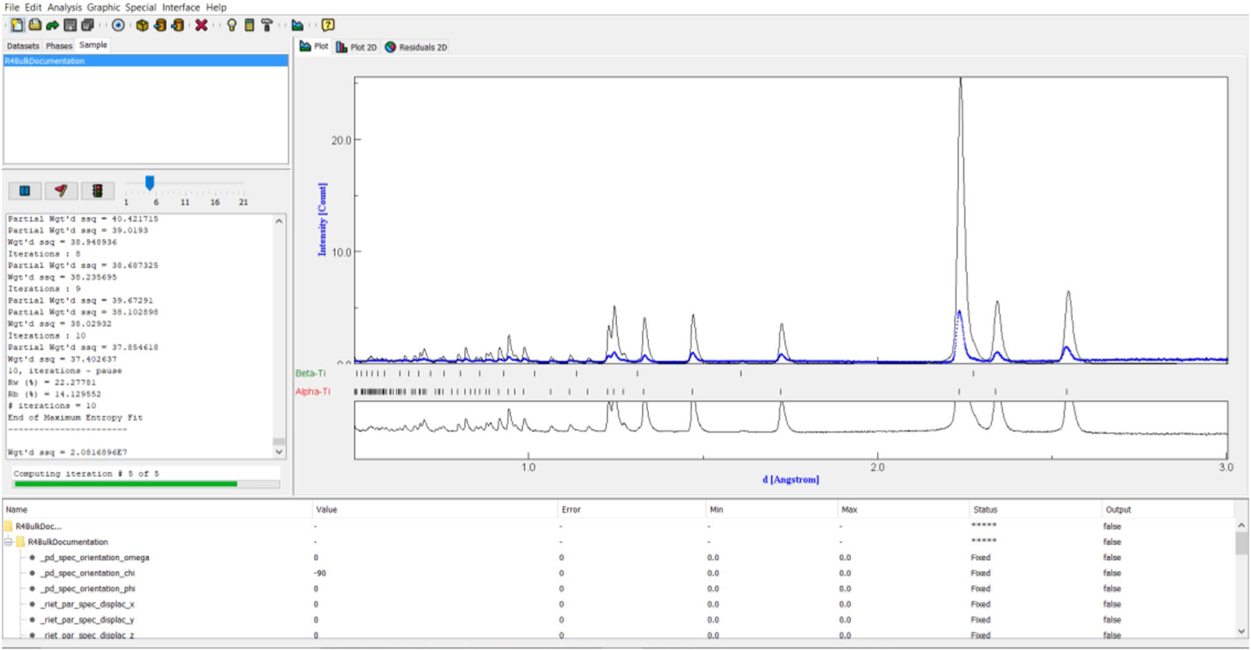
After configuring all parameters as described in Supplementary Material: Refinement Setup, the first refinement cycle was started by selecting the hammer icon (or CTRL + R). This command will trigger output in the text window on the left side of Fig. 6, a refinement status bar appearing below the said text window, and the gradual appearance of a calculated spectrum (blue line) in the spectrum window.

Fig. 6.

Example in-progress refinement demonstrating the refinement status bar, text window with refinement dialogue, refined spectra after the first iteration, the deviation window, and the parameter list. Note the initially poor match between the experimental and calculated spectra after the first iteration

The calculated spectra initially appeared to poorly fit the experimental spectra, but later iterations within the same cycle will address this issue. An example of how the spectrum evolved can be seen comparing Figs. 6 and 7.

Fig. 7.

An improved calculated spectrum observed at a later iteration within the first refinement cycle shown in Fig. 6

When the refinement command is issued, a slider above the text window will appear for controlling how many iterations are performed per cycle. The authors used the default value of five iterations per cycle. Users should perform their own processing experiments to validate if a different number of iterations is better for their datasets or MAUD version.

If the diffraction spectrum appears differently than that seen in any figures so far, check if a linear scale is used for the Y axis (via Graphic → Plot Options and select Linear for the scale mode (first option)). Some installations default to a plot that uses the square root of intensity (Y axis). The authors found a linear scale enabled more detailed tracking of peak fitting than the square root or other scale modes, but this is also a matter of user preference.

It is a good practice to save the analysis after each refinement cycle as a separate.par file (MAUD data format). This will enable troubleshooting, reversion if issues are encountered later in the refinement, and easier collation of refinement parameters (e.g., microstrain, crystallite size), in case they are of interest for later documentation. Suggested information to include in the filename (or other metadata capture method) is: which cycle this file represents, any critical parameter adjustments, and date of refinement.

Evaluating Rietveld Refinement Values

After the first refinement cycle has been completed, a number of process specific values and output quantifications (e.g., texture or phase fraction) can be used to evaluate the quality of the refinement cycle. In this documentation, plots of the experimental and calculated diffraction spectra, phase fractions, crystallographic texture, and R-values from the minimization process are all evaluated. The concept of R-values is discussed briefly below, before looking at the rest of the first cycle’s outputs, and all aforementioned plots/values are evaluated later. These outputs can be used to gauge when a refinement is finished or is improving, as nominally spectra plots will change minimally and the aforementioned values will stabilize when a refinement is near convergence. Many other values or parameters of the model function can also be tracked, but these were the ones focused on in this work.

Most refinement parameters of the model function will report error ranges, along with the refined values. These error values are measures of estimated standard deviations (e.s.d.’s) of the fitting process, and not from any systematic errors due to uncaptured phenomenon. As a result, errors are only reported as the precision of refined parameters, and not the accuracy, as the true value is unknown. Input values that are not refinable will not return e.s.d’s [14, 15].

Identifying when a refinement process is done is highly ambiguous, as no definitive criterion defines when a refinement process is finished. It is highly unlikely a refinement is complete after one cycle, but a thorough investigation of these parameters is still recommended after every cycle. The “best” refinement result may be achieved when the output window indicates that convergence has been reached, or be presented implicitly by achieving the best peak fitting and “best” parameter values for a certain number of refinement cycles. To aid with this assessment, a series of analytical values intrinsic to the minimization process itself are presented at the end of a refinement cycle. The most common of these are known as R-values, which are one measure of how effective the minimization process has been carried out.

R‑Values and Other Parameters

Several different R-values are reported in MAUD after a refinement cycle. The most commonly interpreted R-values are R_w (weighted) and R_exp (expected). R_w (or R_wp as found in other outputs of MAUD) is directly reported in the MAUD text window, while both R_w (R_wp) and R_exp can be found in a cycle’s.LST file formed after pressing CTRL + M post-completion of the refinement cycle. These both convey the “goodness” of a Rietveld fit and generally decrease as a peak fit becomes better.

R_wp (R_w) is calculated by the equation:

$$R_{wp}=\sqrt{\frac{{\displaystyle {\sum }_i{w}_i{\left(y_{C,i}-y_{O,i}\right)}^2}}{{\displaystyle {\sum }_i{w}_i}{\left(y_{O,i}\right)}^2}}$$

where y_C,i = Calculated intensity for a given data point. y_o,i = Specific intensity for a given data point as measured by detector.

And w_i is defined as:

$$w_i=\frac{1}{{\sigma }^2\left[y_{O,i}\right]}$$

And σ is defined as the standard uncertainty for a specific intensity value, y_o,i. σ is defined as the uncertainty of measurement associated with measuring a given diffraction intensity (Y axis of a spectra plot), if the actual value was exactly known. If σ is less than one in value, then the weighted value for the corresponding data point will dramatically increase with a smaller denominator and correspondingly decrease R_wp.

R_exp is defined by a similar equation to R_wp:

$$R_{exp}=\sqrt{\frac{N}{{\displaystyle {\sum }_i{w}_i{\left(y_{O,i}\right)}^2}}}$$

Here, N is defined as the amount of statistical overdetermination. This value is insignificantly different than the total number of data points however, and this latter definition is often used for simplicity [14].

Another parameter, the Le Bail intensity extraction, relates the crystallographic fit to the peak fitting during the refinement process and also gauges the “goodness” of the current refinement fit. If the Le Bail intensity extraction is similar in value to the R_wp value, then the refinement can no longer improve the fitting of crystallographic texture, but improvements to the refinement fit can be made (peak fitting and background). Conversely, if the Le Bail fit is better than R_wp, then the crystallographic texture fitting has potential errors and adjustments to the ODF calculation process are required [16].

Previous work has shown that “R” values may increase erroneously, for instance, when removing background functions [16]. Despite visual inspection confirming the fit was far from “good,” the “R” values were reduced by 10% with the removal of the background function. As both R-values rely on the intensity of a given data point for evaluation, high backgrounds not accounted for by a polynomial or other function will decrease R-values by increasing the value of the squared denominator. Similar trends can be seen with other values, such as “Wgt’d ssd” (weighted sum of squares), where the qualifying parameters report a consistently lower value and thus numerically indicates a better fit, but visual inspection may convey a different story.

The Le Bail intensity extraction parameter was not utilized in this work, due to comparable data being provided by EBSD to confirm the refined texture. For datasets without other data for confirmation however, this parameter is another useful tool in evaluating the “goodness” of a refinement fit and the accuracy of the fitted crystallographic texture. Further discussion on this parameter and others previously identified can be found in literature [16].

Properly Evaluating a Refinement Cycle

It is generally considered best practice to utilize both parameter and visual inspection of the model spectra in determining the quality of a refinement. Again, the qualifying parameters previously discussed will generally decrease in value as refinements improve and should change minimally once the peak fit is “good.” This improvement should be confirmed with visual inspection of all peaks of interest, the spectra difference window, and evaluations of texture and phase fraction.

In the case of peak fitting, the calculated and data spectra should match well with no obvious errors throughout all databanks. Some compromises may be required (e.g., matching high intensity peaks in some databanks while not in others), given the least-squares minimization process may sacrifice some peaks and specific databanks may have an outsized affect in this regard.

These results can also be deemed “good” by verifying if texture and phase fractions converge with previous refinements, or increase after reaching a minimum (indicating the previous refinement was the best possible fit given the current parameters). Similar trends should also be observed for the refinement parameters (e.g., R-values and Wgt’d ssd), but a separate evaluation of this should be completed. Regardless, once both inspection parameters agree, a refinement can be deemed “finished.”

Even when both visual inspection and qualifying parameters indicate the same “goodness,” the results generated by a refinement may still be inaccurate. The authors have found that MAUD, like other refinement software, has issues separating partially overlapped peaks, primarily when considering small phase fractions. Broadening of one peak into the d-spacing of another may be mistaken for an increased phase fraction of a second phase, and without sufficient refinement of polynomial background parameters and other values, this will artificially inflate different aspects of the refinement (e.g., 8 × the expected phase fraction). Thus, full contextualization may be necessary to fully qualify any refinement, though this may require outside knowledge about expected phase fractions (e.g., from other characterization work), or other refinements being used as reference data points.

Evaluating the First Refinement Cycle: Calculated Spectra

The refinement window shown in Fig. 8 illustrates the spectra refinement for the first bank file (“PANEL 150 bank omega 0.0”) after one cycle is completed. As a note, the label “PANEL 150 bank” may appear as PANEL 144 in newer versions of MAUD, and will be addressed as such from here on. The first cycle produced a good start to the refinement, other than the differences in peak intensity at larger d-values.

Fig. 8.

Refinement window after one refinement cycle has completed. Note the much-improved fit observed for the spectra, the reduced deviation plot in the lower window, and the clear presence of a secondary β-Ti peak (highlighted in red box)

The spectra produced by other detector banks can be compared in Fig. 9. Each detector bank has distinctly different spectra. The fit for the 144° bank is good everywhere but the high intensity peaks, while the 90° bank has poor fits near the high intensity peaks and the background at higher d-values (indicated by the rising portion of the spectra on the right side of the spectra window). Fits for the 40° and 120° banks are similarly poor for the background at higher d-values. In addition, the 40° bank has a poor fit for intensity on most peaks, and the 120° bank has over-estimated the highest intensity α-Ti peak. Meanwhile, the 60° bank has under-estimated the smaller peak intensities and over-estimated the highest intensity α-Ti peak.

Fig. 9.

Example spectra showing differences in refinement fit between all detector banks for the same cycle shown in Fig. 8. Regions of poor fit are highlighted in red

A small β-Ti peak can be discerned in Fig. 8. This peak was only present when the lattice parameters for both phases were fixed during this step. The least-squares minimization process can easily find a solution where this peak is not captured, but the overall difference of the refinement has been minimized given the applied parameters. This demonstrates the importance of having knowledge of lattice parameters before using MAUD, particularly for multi-phase materials. Other detector families displayed slightly different patterns with a wide range of fit qualities, due to the different interaction events that give detectable diffraction to each detector family [1–3].

Each family of detectors should be checked to evaluate how the data are fit and inform the status of the initial cycle. Differences between spectra in the same spectra family (e.g., the 144° bank at 0° and 60° rotations) can also be observed, but these are typically smaller than comparing between families. An example of these differences can be seen in Fig. 9. This variation arises from the least-squares minimization for each databank evolving differently to the varying diffraction profiles and the different diffraction events detected by each detector bank. Consequently, alterations to one primary refinement variable may not produce universal improvements across all databanks, and some experimentation in which parameters to refine or fix may be required. In this step, the observation that most banks have places of poor fit indicates more cycles should be completed.

Users may encounter a series of notifications in the refinement text window about “cholesky negative diagonals.” These notifications indicate a given parameter that was unable to be refined further with the initially provided conditions. They do not indicate a refinement that has gone wrong; they indicate when fixed parameters are requested to change in value, but cannot because of this designation. The associated.LST file includes which parameters caused these messages.

Evaluating the First Refinement Cycle: Phase Fractions

The phase fraction values were checked after the first cycle (found in the panel displayed in Fig. ESM 21 (Supplementary Material) in the “Phase” window). Following the first refinement, the initial phase fractions of each phase were refined to values of 0.9730911 for α-Ti and 0.02690888 for β-Ti. These did not deviate significantly from the input values of 0.975 and 0.025.

If a peak for a phase with a small phase fraction, such as the β-Ti peak highlighted in Fig. 8, is not adequately captured or is refined to artificially high intensities, replacing the value for the phase fraction can address this issue. After entering a new value, but prior to starting a new cycle, use of the “Compute Spectra” (CTRL + M) command will regenerate the calculated spectra. Users can iterate with new values and monitor the spectra display to determine if the issue has been resolved. Unless the refinement flag is changed, the phase fractions will be refined in the next refinement cycle, and it may be necessary to fix phase fractions if the refinement continuously deviates from matching the experimental data. Check all of the detector bank families to identify if phase fraction values may have been poorly fit after each cycle.

Evaluating the First Refinement Cycle: Texture

After completing the first cycle, the texture fit was checked. The first step was to pull up the window seen in Fig. 10 by clicking selecting “Graphic → Texture Plot” (CTRL + T), and then selecting which hkl planes and phase to plot, as well as any other plotting options. While several different plot types can be selected, this work evaluated texture using pole figures on a scale of multiples of uniform random distribution (m.r.d.). Once all desired planes are selected (determined by the objective of the study and best practices set by literature), click on “Plot” to set the intensity range, as seen in Fig. 11a. Example calculated textures for the α-Ti phase are shown in Fig. 11b. Additional scans and EBSD data were used to check the fitted texture [11].

Fig. 10.

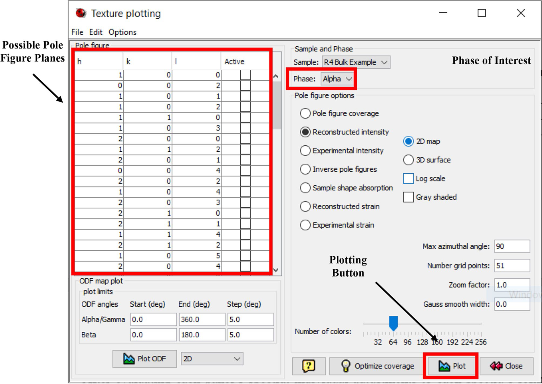
The texture plotting window with all possible planes of interest and phase of interest options

Fig. 11.

Plot intensity range window with the calculated “suitable” range entered as default a and the corresponding pole figures for α-Ti b. These demonstrate a weak to moderate texture of the {0002} poles. Note the three-index notation “equivalent” used in the software for the HCP planes in MAUD

The texture plotting window does not use Miller-Bravais notation for HCP crystal structures. Instead, the software uses the Miller indices notation “equivalent,” which requires conversion (e.g., h + k = −i).

The intensity range values default to the minimum (Min) and maximum (Max) value for all of the pole figures selected. Users can change the range as required to a common scale for comparison of texture between cycles, or leave them as generated for a quick evaluation of texture in the refinement process. The Max value gives an idea of how textured a material is and can indicate poor fitting (e.g., if divergence has occurred and led to unreasonably high values of 20 × m.r.d.). Selecting “Accept” will generate the pole figures specified in Fig. 10 and demonstrated in Fig. 11b.

The pole figure window displays a range of m.r.d. to define the coloring scheme of the pole figures. Other coloring schemes are possible for color-blindness or publication considerations. For reference, a moderate texture was defined as starting at ≈3–4 × m.r.d. The minimum and maximum texture intensity values were recorded, as they can be another marker for when a refinement is complete or running into errors during processing.

The E-WIMV algorithm can diverge after reaching an initial convergence if the status message stating “Convergence reached” is overlooked in the text display window. This divergence will only occur if another refinement is carried out beyond this point (see Example Refinement 2). Thus, the authors evaluated the texture after each cycle to double check this notification was not missed.

Some datasets may benefit from resetting the ODF after the first cycle. This is due to the ODF calculation relying on poorly fitted spectra during the first refinement cycle. Artifacts from the initially fitted data of the first cycle may exist, and continuing to refine the subsequent ODF will propagate these artifacts into later cycles. The authors did not find this issue in developing this tutorial dataset, but other datasets may benefit from resetting the ODF after the first cycle. For samples with high texture, an increased ODF resolution may also be useful.

Evaluating the First Refinement Cycle: R‑Values

These numbers can be found in two locations: the textbox of the refinement window and the.LST file associated with a given refinement.PAR file. The R-values in the refinement are located roughly $\frac{1}{10}$ of the way down from the head of the associated.LST file, as seen in Fig. 12b. Figure 12a demonstrates the textbox seen for the refinement completed in Fig. 8. Here, the R and R_w values are all displayed after pressing CTRL + M once more. R_nb and R_wnb are the same respective values as R and R_w, but calculated without the background being included. Evaluating the presented numbers shows the initial refinement is “good,” with R-values between and below the range of 5–15% [2].

Fig. 12.

Example R-values for the first refinement cycle completed, as seen in Fig. 8 (a), and R-values as reported by the.LST file b. Note these numbers are the same in both figures, but the value in MAUD is given as a percentile

The authors continued with more refinement cycles to see if these values decreased further. One refinement typically is not enough to reach the “best” R-values, but these initial values were promising.

Observations About the First Refinement Cycle and Changes for the Second Cycle

As Fig. 9 shows, three out of five detector families demonstrate incorrect background intensities at high d-values. The majority of detector families also have issues matching peak intensities, an issue that can stem directly from background functions, phase fractions, or other phase parameters. As background functions influence all aspects of a refinement, these were considered most important to modify for the second refinement cycle. Ten additional polynomial background refinement functions were added to each detector bank, as seen in Fig. 13. Adding background functions can be completed by selecting the “Add Parameter” button on the left side of the screen. This window is the same as seen in Fig. ESM 28 (Supplementary Material).

Fig. 13.

PANEL 150 bank with no rotation and 10 additional background parameters added

Any background functions added will be “Fixed” and default to a value of zero. Background parameter values must be changed to refined, as described earlier, once all background parameters have been added to all detector banks.

Ten additional background parameter values are by no means a constant number of background parameters to include for all analyses; this was the value employed in this work and was shown to give good results in prior investigations. Each detector bank may also require a different number of background parameters, depending on the data collected, and is left to user discretion. Datasets with greater quantities of two phases may need less polynomial variables, lest the background function may begin fitting peak data. The addition of background parameters to every detector bank can be a tedious process, but it was effective to overcome issues in peak fitting in this work. Be sure to have saved the previous refinement file before adding in additional polynomial functions, to avoid restarting the refinement process from scratch and enable easy troubleshooting.

Other types of background parameters (e.g., Eta dependent) can also be added, but the authors found consistent success with polynomial background functions. Interpolated backgrounds can be used to fix refinements for which the polynomial functions do not capture high background levels, but these can have unintended effects for some detector banks. Thus, these should only be used as a last resort if restricting the d-range did not address the issue.

Starting a Second Refinement Cycle

After evaluating the fitting of experimental peaks, reported R-values, generated pole figures, and applying refined background polynomial functions, a second refinement cycle was carried out. Other than the addition of background parameters, all other refinement parameters were left the same as output from the first cycle.

Before beginning the second cycle, make sure to press CTRL + M once again to enable the calculation of the freed polynomial background parameters. Then press CTRL + R and wait for the cycle to finish.

Some users may find it advantageous to add background parameters before even the first cycle, but this was not tested in this work.

Evaluating the Second Refinement Cycle: Calculated Spectra

Having completed the second refinement cycle, the various detector banks, texture, phase fraction, and R-values were inspected to determine the quality the refinement.

Figure 14 shows that adding polynomial background functions partially improves the overall fit of all banks. The poor background fit at large d-spacing is still present in the 60° and 40° banks, but the profile fit does seem to improve. The poor fit for the secondary β-Ti phase in the 144° bank was also observed. The secondary phase matching of the 120° bank seems improved; however, ideally both banks would match the secondary phase for the most consistent refinement result.

Fig. 14.

Detector bank spectra following the second refinement cycle. Note the partially improved background fit and the missing β-Ti peak in the 144° bank, but the improved fit in the 120° bank

Some detector banks appear to match all peak intensities, while others do not. This has been shown to have a minimal negative impact on texture results generated from MAUD for the datasets processed in this work, but this may not be the case in other datasets.

The inconsistent background at higher d-spacing may pose an issue later in the refinement. From least-squares minimization, the software will minimize the difference criterion of all data points, a process weighted toward areas with a larger number of data points (i.e., the background). This can sacrifice fit quality in the peak regions. Though this effect cannot be directly quantified, visual inspection of the peak fitting shows such an effect may be present, primarily regarding the fitting of the β-Ti peak. It is up to the user to determine when such an effect is appropriately minimized, or if removing this specific range of interplanar values may be beneficial to the refinement process. For the purpose of this documentation, no further processing was applied to address these high d-spacing background issues, as this was found to not be the direct cause for reduced peak fitting.

Evaluating the Second Refinement Cycle: Phase Fractions

The poor fitting of the β-Ti phase peaks when inspecting the spectra suggests a potential issue with the refinement’s calculated phase fraction. As Table 1 shows, the β-Ti phase fraction value increased in this cycle. However, the β-Ti crystallite size is substantially reduced, likely leading to a broad peak profile.

Evaluating the Second Refinement Cycle: Texture

Pole figures evaluated in the second cycle are shown in Fig. 15a. The second cycle increased the maximum intensity of the experimental texture (Fig. 15b), while the pole figures are relatively unchanged in character.

Fig. 15.

Updated pole figures of α-Ti (a), updated texture intensities (b), and R-values generated from the second refinement cycle (c). Note the decreased R-values, as compared to Fig. 12

Evaluating the Second Refinement Cycle: R‑values

Figure 15c shows that the refinement R-values have decreased in value. This, along with other evaluations from spectra and texture, indicates that the refinement is improving by traditional metrics.

Observations About the Second Refinement Cycle and Changes for the Subsequent Cycles

With no apparent changes to any parameters required after the second cycle, no other background parameters or alterations to values were performed. Several further refinement cycles were performed to cause the refinement to converge and identify if further cycles could address the issues observed with the β-Ti peak.

Users should save their second refinement as a distinct. PAR file and complete further cycles.

Starting Subsequent Refinement Cycles

Eight additional cycles were run to evaluate how parameters changed with further refinement. Cycle 3 is detailed below, and cycles 4 and 5 are discussed in Supplementary Material. The texture max/min, β-Ti phase fractions, and R-values for subsequent refinement cycles are summarized in Table 1 for brevity. Following the same evaluation process as before the peak profiles, phase fractions, texture, and R-values were evaluated.

Evaluating the Third Refinement Cycle: Calculated Spectra

Figure 16 shows that the peak profiles after the third cycle seem relatively unchanged with the exception of the 144° bank. The 120° bank continues to be well matched for both phases, while the 144° bank struggles to capture the β-Ti profiles.

Fig. 16.

Detector bank spectra following the third refinement cycle. Again, note the reduced fitting in the 144° bank of the β-Ti

The loss of the β-Ti peak brings up an important detail. Low phase fractions of secondary phases may be difficult to fully resolve in the refinement process and can cause refinements to diverge unexpectedly. Taking note of refinement changes, such as the decrease in β-Ti, may indicate when a refinement is approaching or has passed official (declared by the software) or implicit convergence (implied by evaluating the various parameters).

Evaluating the Third Refinement Cycle: Phase Fraction

A noticeable drop in the β-Ti phase fraction from 3.50 vol% to 2.72 vol% was observed, indicating that the refinement process may be inaccurately capturing phase fractions after the third cycle.

Evaluating the Third Refinement Cycle: Texture

Figure 17 shows the intensities and pole figures appear about the same as Fig. 15. A much smaller increase in maximum m.r.d. was observed after the third refinement cycle, suggesting convergence may be near for this refinement process.

Fig. 17.

Texture intensities (a) and updated pole figures (b) of α-Ti generated from the third refinement cycle. Note the slightly increased intensities

The reduced peak fitting of the second phase, however, suggests these results may not be as accurate as desired.

Evaluating the Third Refinement Cycle: R‑Values

In a similar fashion to the texture results, limited but noticeable improvements in the reported R-values can also be seen, as observed in Fig. 18. Note again that “Rw” is equivalent to “Rwp” and “R” equivalent to “Rp” in the LST files.

Fig. 18.

R-values of the second cycle (left) and the third cycle (right). Note the general, but gradual, improvement of the R-values, suggesting convergence is close by traditional metrics

Observations About the Subsequent Refinement Cycle and New Campaign

Table 1 shows that the texture maximum returned to values closer to those seen during the second set of refinement cycles, while the R-values gradually improved as the number of cycles increased. Thus, it appears at first glance that the refinement has overall improved after ten cycles. MAUD may never reach convergence with this dataset, and users may find these results satisfactory, given their limited change per cycle.

However, looking at the spectra, this series of refinement cycles has become worse at capturing the experimental results. After the first refinement cycle, all refinements reduced the secondary phase peak fitting, even with increased β-Ti phase fractions (Fig. 19). Thus, the fitting of the β-Ti phase decreased in accuracy. The calculated spectra also changed minimally after the second refinement cycle, because the least-squares minimization was unable to match the calculated spectra as configured. The expected β-Ti phase fraction is approximately 3 volume %, and was shown to fall below this value at the same point β-Ti peak fitting was reduced. As a result, this series of refinements was designated as partially inaccurate.

Fig. 19.

Comparison of the peak fitting for the secondary β-Ti phase after the first and second refinement cycles in the “PANEL 150 Bank Omega 0.0” datasets. Note the gradual reduction in overall secondary phase peak fitting, despite the improved R-values reported in Fig. 18

Given the poor fit of the 144° β-Ti phase peak and the data in Table 1, the authors reverted to the output of the first refinement cycle and fixed the phase fraction. The poor fit is likely due to the least-squares minimization evaluating other data banks that do not have a defined β-Ti peak at this location. Consequently, the least-squares minimization with the lowest difference for all detector families will not include the β-Ti peak, thereby removing this fit from the 144° detector family. Fixing the phase fraction prevented this minimization from happening.

This series of initial refinement cycles shows the importance of acknowledging all aspects of Rietveld refinement, as no single attribute can wholistically determine when a refinement is the “best” that it can be. Different datasets will also require different processing (e.g., some may reach convergence as dictated by the software, while others may never converge, as highlighted here, requiring user interpretation).

Modified Second Refinement Cycle: Fixed Phase Fractions

To counter the reduced peak fitting and phase fraction inaccuracy, a new refinement campaign with fixed α-Ti and β-Ti phase fractions was performed. This campaign uses the first cycle from the previously described initial campaign, and then fixes phase fractions before starting a (modified) second cycle. The authors thus reverted to the first refinement cycle output and fixed the phase fraction, as indicated in Fig. 20, with the red fill color for the text box.

Fig. 20.

Fixing refinement values in the second refinement cycle file

Restarting from the results of the first refinement cycle underscores the importance of storing each previous cycle, as it can be advantageous to return to a previous file in case one processing pathway deemed a poor fit.

Evaluating the Modified Second Refinement Cycle: Calculated Spectra

Fixing the phase fraction from the first refinement cycle has improved the peak fitting. As seen in Fig. 21, all detector banks have improved in peak matching, while also maintaining the secondary β-Ti phase peaks in the 120° and 144° PANEL banks.

Fig. 21.

PANEL bank spectra following the modified second refinement cycle. Note the presence of the well-defined secondary phase peak in the 144° bank

Evaluating the Modified Second Refinement Cycle: Texture

Figure 22 shows the same texture profile in the generated pole figures, but does have a noticeably reduced maximum intensity. The different numbers here (differences of ≈0.1 multiples of uniform random distribution from the second refinement cycle in Fig. 15) suggest the previous refinements with a refinable phase fraction were less representative of the experimental data. This difference is negligible in the grand scheme of analysis, but still underscores how small changes to the refinement process can have clear effects.

Fig. 22.

Texture intensities (a) and updated pole figures (b) of α-Ti generated from the second fixed phase fraction cycle. Note the decreased m.r.d. value, as opposed to those listed in Table 1

While maximum texture intensity is not the most reliable way to evaluate crystallographic texture within a material, within MAUD it is used as a general gauge of “goodness of fit.” Different texture intensities, though less than 1 m.r.d. in difference, still indicate a different path evolution of the least-squares minimization.

Evaluating the Modified Second Refinement Cycle: R‑Values

Figure 23 compares the R-values for the modified second refinement cycle (fixed phase fraction) and those from the original second refinement cycle (using a refinable phase fraction). Though the values are fairly comparable, the refinable phase fraction seems to produce a “better” fit (lower R-values) than that of fixing the phase fraction. As previously noted, peak fitting should also be a key consideration for evaluating if a refinement is in fact “better”; here, the difference in R-values is not reflective of the actual quality of the refinement.

Fig. 23.

R-values for the second cycle with fixed phase fractions (left) and the second cycle with refinable phase fractions (right)

Observations About the Modified Second Refinement Cycle and Changes for the Third Cycle

With all of these considerations in mind, another refinement cycle with fixed phase fractions was carried out. As the fit visibly improved in the spectra, the texture may also be more representative of the actual results. An additional cycle was completed to confirm this hypothesis.

Third Modified Refinement Cycle: Fixed Phase Fractions

Carrying out a third cycle with fixed phase fractions produced the following text window message observed in Fig. 24. Here, MAUD could not refine parameters more than it already had with the fixed phase fractions and reached an “official” convergence.

Fig. 24.

Refinement message indicating convergence has been reached before the cycle was completed

Users can still evaluate the spectra, texture, and R-values to ensure all aspects of the refinement are still “good.” Continuing to refine past the convergence event generates artificial results not representative of the experimental data. An example can be seen in the second detailed instructional set listed in the Online Appendix.

The convergence message may reside several lines above the bottom section of text displayed in the refinement text window. Users can easily miss the notification of refinement convergence, and accidentally continue to refine past a notification of a convergence endpoint. Thus, users should always take note of the end-position of the refinement status bar and scroll up slightly in the text window to check for the below message.

Evaluating the Modified Third Refinement Cycle: Calculated Spectra

Despite a fixed phase fraction and having officially reached convergence, the updated spectra in the third fixed phase fraction refinement cycle worsened for the 144° bank. This change is only for the 0.0° bank dataset, and not for the 67.5° and 90° (Fig. 25). Regardless, these differences suggest that the refinement’s official software designated convergence was actually a worse refinement than that of the second refinement cycle with a fixed phase fraction. Consequently, the second refinement output appears to be the point of implicit convergence and the most representative. This can be further validated by comparing the generated pole figures.

Fig. 25.

Peak profiles from the 144° PANEL bank datasets, showing differences in quality of peak fitting. The 0.0° omega dataset (top) demonstrated a worse fit for the secondary phase peaks, while the 67.5° (bottom left) and 90.0° (bottom right) maintained adequate profiles observed from the second fixed phase fraction refinement

Evaluating the Third Modified Refinement Cycle: Texture

The texture intensity range and pole figures are shown in Fig. 26. The maximum intensity has jumped a noticeable amount (≈ 0.2 m.r.d.), again approaching the intensities observed in Fig. 17. Given these refinements demonstrated poor secondary phase peak fitting and had increased texture intensities, it is not surprising this phenomenon is also observed.

Fig. 26.

Texture intensities (a) and updated pole figures (b) of α-Ti generated from convergence in the third fixed phase fraction cycle. Note the noticeable jump in maximum intensity

Though the mechanisms by which this shift in values has occurred are not known (e.g., internal error in parameter calculation or mis-representation of diffraction data in the refinement window), these differences indicate that the second refinement cycle with fixed phase fractions produces the better overall refinement.

Evaluating the Third Modified Refinement Cycle: R‑Values

As shown in Fig. 27, the R value decreased slightly from the modified second cycle, but the R_w value remained the same.

Fig. 27.

R-values for the third fixed phase fraction refinement cycle where convergence was reached

Observations About the Modified Third Refinement Cycle

With the objective of this refinement process to be the calculation of crystallographic texture data from diffraction spectra via a repeatable processing routine, these results and the refinement outputs/status indicate this objective was met. All refinement outputs have been analyzed, and an implicit convergence point has been reached from their evaluations. Despite the decreased R-values as compared to those from the modified second cycle, the texture and peak fitting evaluations indicate that this cycle may not be the best fit. The modified second refinement cycle was used for evaluating crystallographic texture, and this approach was used in all samples described in [11].

With other datasets, the user must determine when a refinement process is complete. Although it is desirable for MAUD to officially reach convergence and notify the user accordingly, this may take well over 10 cycles to complete, or may never occur, depending on the experimental spectra loaded. The user also needs to be cognizant of refinement results being less accurate than previous refinements, as demonstrated here.

An implicit convergence may be reached after seeing minimal output changes over several refinements, or may be reached by noting undesired deviations with a given assessment point, as previously demonstrated. Thus, users will have to determine when their own data are sufficiently processed for their own experimental objective (e.g., calculating texture intensities versus changes in texture profile).

There are additional refinement paths that could be explored for additional accuracy. For example, if the crystallite size of the β-Ti was fixed, this may have permitted further refinement of the value with a refinable phase fraction. The number of background terms could also be investigated more systematically, or additional function types explored. Allowing the lattice parameters to vary in a narrow range may have also improved some fitting, but the present outputs were deemed sufficient, especially when compared to data collected from other sources.

Independent Verification of the Textures and Phase Fractions

The primary reason of this work was to generate a consistent operating procedure when using MAUD for evaluating crystallographic texture across a series of samples. The pole figures generated from the modified second refinement cycle are compared to a set of pole figures generated by large-scale EBSD in Fig. 28. The two sets of pole figures represent the same hkl planes, despite MAUD reporting plane normals in three-index notation and MTEX in four-index notation. These EBSD maps evaluated the same regions of α-Ti studied using neutron diffraction over a 4 mm × 4 mm area with a 1 μm step size. Measurements were made with a LEO 1525 FESEM at the National Institute of Standards and Technology in Boulder, Colorado. Data from the EBSD measurements were processed using the TSL OIM Data Collection software version 7 and the MATLAB plug-in MTEX version 5.2.7. All pole figures presented are reported in the HIPPO/MAUD sample reference frame.

Fig. 28.

Comparison of MAUD refined α-Ti pole figures (a) and experimental pole figures acquired from large-scale EBSD (b)

Though different coloring schemes were employed between each pole figure, the overall profiles are nearly identical. The same offset centering of the (0002) and ($11\overline{2}0$) pole figures is observed, along with the same profiles and comparable intensities. Two differences are the slight rotation of the EBSD pole figures as compared to those generated using MAUD, and the smearing of the EBSD pole figures. The former is thought to occur due to the EBSD scan evaluating a smaller number of grains (0.00032 mm³ vs ≈600 mm³), and the latter from different processing routines used to generate the EBSD pole figures. Regardless, these results are similar in profile and intensity, directly validating the processing routine demonstrated in this work.

Fits from other cycles reporting lower β-Ti phase fractions were relatively close to experimental data shown in Fig. 28. Intensities of reported texture were within ≈0.2 m.r.d. and demonstrate that these suspect cycles were in fact “accurate” for the purpose of this investigation. The outputs of these cycles could be used for further investigation, but the systematic process employed here guarantees confidence in the calculated results.

When analyzing data generated from large interaction-volume techniques (e.g., neutron diffraction), comparable studies of crystallographic texture on the same sample are challenging to complete with other techniques (e.g., laboratory XRD or electron back scatter diffraction (EBSD)) and may require extensive parallel efforts.

The differences between these results underscore the importance of maintaining the same refinement processing scheme. Other datasets may be less forgiving in texture deviations reported from refinements with reduced secondary phase fractions, drastically altering the interpretation of experimental data.

The reduced β-Ti refinement cycles may have also been close to EBSD results, but due to the limited secondary phase fraction of the β-Ti (≈ 3% volume fraction), this was difficult to evaluate. This small constitution would have minimal effects on parameter values after the initial refinement, and thus cause the macrotexture results to deviate by a “tolerable” amount. In materials with similar phase fractions, this constitution may become a much larger issue. A hint of this can already be seen by the noticeable shift in texture intensities as a response to changes in the calculated volume fraction of β-Ti. This shift in β-Ti content once more underscores how monitoring peak fitting is always key to an effective refinement, regardless of refinement parameter outputs.

Streamlining an Analysis Process

One last area of instructional insight is on streamlining the analysis of related datasets in MAUD. For experimental files obtained from diffraction experiments completed sequentially (e.g., local measurements all completed within the same sample insertion of the HIPPO beamline), a constant set of refinement conditions for processing of texture information is important. Allowing MAUD to refine calibration values for every refinement injects uncertainty into any data or understanding gleaned from the software, and should be avoided. Human error in file or parameter input may also pose an additional threat to refinement quality. Calibration values, known in shorthand within MAUD as “difc” parameters, are the “constant” diffraction condition values for a given sample position. For experiments where only the Z-position of the sample was changed (no removal of the sample from the sample holder), the diffraction conditions should be the same in the XY-plane. Changing or letting these parameters refine independently during different refinement processes will produce different, possibly incorrect or inconsistent results between refinements and should be avoided. Though these effects may be small, all sources of uncertainty should be mitigated, whenever possible.

A Linux-based program called prepare_maud.sh, which copies the current state (parameters, ODF, etc.) of a previously completed refinement into another fresh file, is available by asking the beamline scientist you are working with. The newly generated file is exactly the same as the previous one, with the exception of the dataset being used. These are switched out via the generated script. This enables the calibration values (designated as “difc” within MAUD) to be held constant between different runs and ensures all refinements are completed with the same basic constants. To facilitate this process, the authors completed a refinement generally representative of each sample. This specific dataset could originate from a bulk experiment, or the most representative scan of a series of local measurements (e.g., for a given rolling texture).

Users will require a Linux-based computer or virtual terminal to operate the streamlining plug-in, and the free Linux plug-in known as Cygwin was used here. This virtual terminal creates a Linux directory within a given drive and is navigated using the bash shell. The exact fashion in which prepare_maud.sh will operate depends on the set of sequential experiments completed for your work. Regardless, once the difc values have been loaded into a new refinement, users can modify all other parameters as they see fit to continue their refinement process.

Independent of which representative dataset is selected, XRD calculated lattice parameters of the sample should be fixed and used in the initial refinement to calculate consistent and accurate “difc” values. These parameters can then be locked using the TreeTable (Fig. ESM 29, Supplementary Material). This was performed via the “Multi Bank” higher-tier tree level to fix calibration values in bulk groups and streamline the process. Lattice parameter estimates from other works may also be employed here if XRD measurement is unavailable, but these values should be left refinable throughout the first few cycles, as they likely will not perfectly match actual values. It may be necessary if a divergence in peak fitting is observed to fix lattice parameters after a series of cycles; this can be completed in the same process described above.

Users will also want to erase the calculated ODF for the calibration value setting refinement to avoid skewing later refinements into having the same reported texture. This can be completed via the window seen in Fig. 29.

Fig. 29.

The E-WIMV options panel where the button to reset a previously calculated ODF is located (highlighted in red)

The number of cycles required to reach convergence from this process may be less than that of the “conditioning” refinement file (e.g., 1–2 cycles), but trends in diffraction data can still be evaluated.

Conclusions

This work has demonstrated a good-practice guide to evaluating crystallographic texture using the Rietveld refinement software MAUD. Though powerful, the software has over a thousand different parameters, which without careful management by users, can render Rietveld refinements of neutron or XRD experiments erroneous. A step-by-step documentation of each key point in the MAUD refinement process is described, along with areas of troubleshooting previously overlooked in some instructional material.

The following information, if collected before a refinement, can aid the user in guiding the refinement process. These include:

1. Accurate lattice parameters for the material under study from XRD or other technique. HIPPO is not as sensitive to changes in lattice parameters as other techniques such as XRD, and gives better results after starting sequential refinements with fixed experimental lattice parameters. Approximate lattice parameters from prior work may also be left refinable and fixed as need be if direct measurement is unavailable.

   1. To capture changes in lattice parameters, allow lattice parameters to be refinable when refining datasets after completing an initial large scale or bulk refinement. This assumes one carries over the bulk refinement results into other data files using prepare_maud.sh.

2. Determining if a triclinic or orthotropic sample symmetry is more applicable for your expected results. Triclinic sample symmetries should be used for initial processing until sufficient symmetry across your reference frame is observed to warrant an orthotropic sample symmetry assumption.

3. Estimates of the phase fractions of your system. This will help gauge if MAUD encounters issues refining different profile intensities from overlapping peaks (e.g., shouldering in β-Ti and α-Ti).

4. Your material’s Debye–Waller factor. This attenuation factor is sensitive to material composition and can influence your refinement results noticeably, especially regarding phase fraction.

   1. For one phase systems, the Debye–Waller factor can be set as a refinable parameter, but for two-phase systems the Debye–Waller factor should be fixed, and with a value informed by literature, experiments, and/or iterative refinements.

5. Estimates of texture intensity. It is useful to know approximately to what degree a given material will be textured prior to using MAUD. This helps to determine when a refinement is close to completion, but is not mandatory. Careful, repeatable management of one’s processing routine can compensate for not having this prior knowledge.

This work also compared the calculated texture using MAUD to that reported from a parallel study using EBSD. Both processes generated nearly identical texture information, and demonstrated the validity using this instructional set for producing consistent and accurate texture information. Outside texture experiments were also used to demonstrate the importance of acknowledging whether an orthotropic or triclinic sample symmetry is more appropriate for a given texture dataset in Refinement Setup (see Texture and ODF Resolution).

To assist in employing MAUD for other texture studies, a data repository has been created for readers to acquire the files evaluated here and to test the presented processing routine [4]. Instructional documentation, including a detailed step-by-step process on the demonstrated refinement and a different neutron diffraction experiment, is also provided here for user reference. All provided files should be compatible with newer MAUD versions.

The authors hope this work will be of benefit to a wide number of disciplines and users across the scientific spectrum. They also welcome any questions, concerns, or curiosities readers may have.

References

- 1.Lutterotti L, Matthies S, Wenk H-R, Schultz AS, Richardson JW (1997) Combined texture and structure analysis of deformed limestone from time-of-flight neutron diffraction spectra. J Appl Phys 81:594–600. 10.1063/1.364220 [DOI] [Google Scholar]
- 2.Wenk H-R, Lutterotti L, Vogel SC (2010) Rietveld texture analysis from TOF neutron diffraction data. Powder Diffr 25:283–296. 10.1154/1.3479004 [DOI] [Google Scholar]
- 3.Lutterotti L (2000) MAUD tutorial—computing ODF from traditional pole figures using WIMV,10 [Google Scholar]
- 4.Creuziger AA (2021) MAUD-Tutorial Files for “MAUD rietveld refinement software for neutron diffraction texture studies of single and dual-phase materials,” 11 files, 18.7 MB. 10.18434/MDS2-2400 [DOI] [PMC free article] [PubMed]
- 5.Toby BH (2019) Rietveld refinement. In: International tables for crystallography Wiley, Hoboken, pp 344–373 [Google Scholar]
- 6.Matthies S, Lutteroti L, Wenk HR (1997) Advances in texture analysis from diffraction spectra. J Appl Crystallogr 30:31–42. 10.1107/S0021889896006851 [DOI] [Google Scholar]
- 7.Rietveld HM (1969) A profile refinement method for nuclear and magnetic structures. J Appl Crystallogr 2:65–71. 10.1107/S0021889869006558 [DOI] [Google Scholar]
- 8.Rietveld HM (1988) The Rietveld method—a historical perspective. Aust. J Phys 41. http://articles.adsabs.harvard.edu/cgi-bin/nph-iarticle_query?1988AuJPh.41.113R&defaultprint=YES&filetype=.pdf. Accessed 23 March 2020. [Google Scholar]
- 9.Takajo S, Vogel SC (2018) Determination of pole figure coverage for texture measurements with neutron time-of-flight diffractometers. J Appl Crystallogr 51:895–900. 10.1107/S1600576718007732 [DOI] [Google Scholar]
- 10.Toby BH, Von Dreele RB (2013) GSAS-II: the genesis of a modern open-source all purpose crystallography software package. J Appl Crystallogr 46:544–549. 10.1107/S0021889813003531 [DOI] [Google Scholar]
- 11.Saville A, Klemm-Toole J, Vogel SC, Creuziger A, Benzing J, Clarke AJ, Pilchak AL, Nandwana P, Semiatin SL (2021) Texture evolution as a function of scan strategy and build height in electron beam melted Ti–6Al–4V. Addit Manuf 10.1016/j.addma.2021.102118 [DOI] [PMC free article] [PubMed]
- 12.Larson AC, Dreele RBV (2004) GSAS—general structure analysis system, Los Alamos National Laboratory
- 13.Saville AI, Klemm-Toole J, Vogel SC, Kumar SK, Clarke AJ (2019) Texture evolution in Ti–6Al–4V with different scan strategies. Adv Addit Manuf Powder Metall AMPM 2019:667–672 [Google Scholar]
- 14.McCusker LB, Von Dreele RB, Cox DE, Louër D, Scardi P (1999) Rietveld refinement guidelines. J Appl Crystallogr 32:36–50. 10.1107/S0021889898009856 [DOI] [Google Scholar]
- 15.Miyagi L, Merkel S, Yagi T, Sata N, Ohishi Y, Wenk H-R (2006) Quantitative Rietveld texture analysis of CaSiO3 perovskite deformed in a diamond anvil cell. J Phys Condens Matter 18(2006):S995–S1005. 10.1088/0953-8984/18/25/S07 [DOI] [PubMed] [Google Scholar]
- 16.Toby BH (2006) R factors in Rietveld analysis: How good is good enough? Powder Diffr 21:67–70. 10.1154/1.2179804 [DOI] [Google Scholar]
Associated Data
This section collects any data citations, data availability statements, or supplementary materials included in this article.