Testing Mediation Effects Using Logic of Boolean Matrices

Abstract

A central question in high-dimensional mediation analysis is to infer the significance of individual mediators. The main challenge is that the total number of potential paths that go through any mediator is super-exponential in the number of mediators. Most existing mediation inference solutions either explicitly impose that the mediators are conditionally independent given the exposure, or ignore any potential directed paths among the mediators. In this article, we propose a novel hypothesis testing procedure to evaluate individual mediation effects, while taking into account potential interactions among the mediators. Our proposal thus fills a crucial gap, and greatly extends the scope of existing mediation tests. Our key idea is to construct the test statistic using the logic of Boolean matrices, which enables us to establish the proper limiting distribution under the null hypothesis. We further employ screening, data splitting, and decorrelated estimation to reduce the bias and increase the power of the test. We show that our test can control both the size and false discovery rate asymptotically, and the power of the test approaches one, while allowing the number of mediators to diverge to infinity with the sample size. We demonstrate the efficacy of the method through simulations and a neuroimaging study of Alzheimer’s disease. A Python implementation of the proposed procedure is available at https://github.com/callmespring/LOGAN.

1. Introduction

Mediation analysis is an important tool in scientific studies. It seeks to identify and explain the mechanism, or pathway, that underlies an observed relationship between an exposure and an outcome variable, through the inclusion of an intermediary variable, known as a mediator. It decomposes the effect of exposure on the outcome into a direct effect and an indirect effect, the latter of which is often of primary interest and has important intervention consequences (Pearl, 2001). Mediation analysis was first proposed with a single mediator in social science (Baron and Kenny, 1986). In recent years, it is receiving increasing attention, and has been extended to the settings of multivariate and high-dimensional mediators. It is now widely used in a large variety of scientific applications, including psychology (MacKinnon and Fairchild, 2009), genomics (Huang and Pan, 2016), genetic epidemiology (Huang, 2018), and neuroscience (Zhao and Luo, 2016).

In mediation analysis with high-dimensional mediators, a fundamental but challenging question is how to infer the significance of individual mediators. The main difficulty is the sheer number of possible paths that go through all combinations of the mediators. Consequently, the total number of potential paths that go through any mediator is super-exponential in the number of mediators, rendering almost any existing testing procedure ineffective. To circumvent this issue, most existing mediation inference solutions either explicitly impose that the mediators are conditionally independent given the exposure, or simply ignore any potential directed paths among the mediators. Such simplifications substantially reduce the complexity of the hypotheses to test. Adopting this conditional independence assumption, Boca et al. (2014) proposed a permutation test with family-wise error control, while Zhang et al. (2016) proposed a screening-and-testing assisted approach. Huang and Pan (2016) proposed a transformation model and assumed conditional independence for the transformed mediators. Sampson et al. (2018) and Djordjilović et al. (2019) directly tested whether each mediator is independent of the exposure or conditionally independent of the outcome given the exposure, ignoring mediator-by-mediator interactions, while controlling for family-wise error rate or false discovery rate in multiple testing. Whereas these tests have been demonstrated effective in numerous applications, they all ignored potential paths and interactions among the mediators. Even though this strategy may be plausible in some applications, it may not hold true in others. For instance, in our brain imaging mediation analysis study in Section 7, different brain regions are conceived to influence each other. In genetics studies, different genes are expected to interact with each other (Chakrabortty et al., 2018). Actually, such examples are often the rule rather than the exception. Therefore, it is of great importance to develop a mediation testing method that takes directed paths and interactions among the mediators into consideration.

Recently, Chakrabortty et al. (2018) made an important step forward for inference of mediation effects while allowing mediator interactions. They formulated the structure of the exposure, the potential mediators, and the outcome as a directed acyclic graph (DAG). They defined the individual mediation effect of a given mediator as the summation of all the effects of the exposure on the outcome that can be attributed to that mediator. They then established the corresponding confidence interval for their interventional calculus type estimator of the mediation effect. However, the effects along different paths may cancel each other, resulting in a zero individual mediation effect in the summation. Rather than taking average and cancelling out the total effect, we argue this type of mediator is important and should be identified by the inferential test too. See Section 2.2 for more discussion.

There have also been some recent proposals of penalized sparse estimation of mediation effects (Zhao and Luo, 2016; Nandy et al., 2017). In addition, there is a large body of literature studying penalized estimation of directed acyclic graph given observational data (see, e.g., van de Geer and Bühlmann, 2013; Zheng et al., 2018; Yuan et al., 2019, and the references therein). However, estimation is an ultimately different problem from inference. Although both can in effect identify important mediators or links, estimation does not produce an explicit quantification of statistical significance, and does not explicitly control the false discovery. As such, we are targeting a completely different problem than those estimation approaches. More recently, Li et al. (2019) developed a constrained likelihood ratio test to infer individual links or some given directed paths of a DAG. Nevertheless, their hypotheses are very different from our problem of inferring significant mediators.

In this article, we propose a novel hypothesis testing procedure to evaluate individual mediation effects, which takes into account directed paths among the mediators and is equipped with statistical guarantees. A key ingredient of our proposal is to construct the test statistic using the logic of Boolean matrices, which allows us to establish the proper limiting distribution under the null hypothesis. In comparison, the asymptotic properties of the test statistic built on the usual matrix operations are extremely challenging to establish. In addition, the Boolean matrix-based test statistic can be naturally coupled with a screening procedure. This helps scale down the number of potential paths to a moderate level, and in turn reduces the variance of the test statistic, and enhances the power of the test considerably. Furthermore, we use a data splitting strategy to ensure a valid type-I error rate control for our test under minimal conditions on the screening. We employ some state-of-the-art estimator of DAG (Zheng et al., 2018) to form an initial estimator of the directed paths. We also devise a decorrelated estimator to reduce potential bias induced by high-dimensional mediators. Consequently, it ensures the resulting estimator is $\sqrt{n}$-consistent and asymptotically normal. We then employ a multiplier bootstrap method to obtain accurate critical values. Finally, we couple our test for the significance of an individual mediator with a multiple testing procedure (Djordjilović et al., 2019) to control the false discovery rate (FDR) of simultaneous testing of multivariate mediators.

Our contributions are multi-fold. Scientifically, rigorous inference of mediation effects is a vital and long-standing problem. But nearly all existing solutions ignore potential interactions among the mediators. Our proposal thus fills a crucial gap, extends the scope of existing tests, and offers a useful inferential tool to a wide range of scientific applications. Methodologically, our proposal integrates the logic of Boolean matrices, DAG estimation, screening, data splitting, and decorrelated estimation to reduce the bias and increase the power of the test. It is ultimately different from the test of Chakrabortty et al. (2018), which defined the mediation effect through averaging, required the DAG selection consistency, focused on dealing with the equivalence class of DAG estimators, and did not consider multiple testing. By contrast, our method targets a different, and in our opinion, a more general definition of mediation effect, does not require the DAG selection consistency, and mostly focuses on the single DAG situation. We discuss the extension of the test to the equivalence class situation in Section 8. We also compare our test with that of Chakrabortty et al. (2018) numerically, and show our method is empirically more powerful while achieving a valid type-I error control. Theoretically, we systematically study the asymptotic properties of our test, while allowing the number of mediators to diverge to infinity with the sample size. We show that our test can control both the size and FDR asymptotically, and the power of the test approaches one. As a by-product, we derive an oracle inequality for the estimated DAG by the method of Zheng et al. (2018), which is needed to establish the consistency of our test, but is not available in Zheng et al. (2018).

The rest of the article is organized as follows. We define our hypotheses in Section 2, and develop the test statistics based on the logic of Boolean matrices in Section 3. We propose the testing procedures in Section 4, and investigate the asymptotic properties in Section 5. We present the simulations in Section 6, and a neuroimaging application in Section 7. We conclude the paper in Section 8, and relegate all proofs to the supplementary appendix.

2. Hypotheses

In this section, we first present the Gaussian graphical model, based on which we formulate our mediation testing problem. We then formally develop the hypotheses we aim to test, and compare with the alternative formulation in Chakrabortty et al. (2018).

2.1. Gaussian graphical model

Consider an exposure variable E, a set of potential mediators M = (M₁,…,M_d)^⊤, and an outcome variable Y. Let X = (E, M^⊤, Y)^⊤ collect all the variables, and assume X follows the linear structural equation model,

$$X-{\mu }_0=W_0\left(X-{\mu }_0\right)+\epsilon ,$$ (1)

where μ₀ = E(X), W₀ is the (d + 2) × (d + 2) coefficient matrix, and ε = (ε₀, ε₁,…, ε_d+1)^⊤ is the mean-zero vector of errors. The matrix W₀ specifies the directional relationships among the variables in X, which can be encoded by a directed graph. Let X_j denote the (j + 1) th element of X, j = 0,…,d + 1. For i, j ∈{0,1,…,d + 1}, if X_i is a direct cause of X_j, then an arrow is drawn from X_i to X_j, i.e, X_i → X_j, and W_0,j,i ≠ 0. In this case, X_i is called a parent of X_j, and X_j a child of X_i. For an integer k ≥ 1, a k-step directed path between X_i and X_j is a sequence of distinct nodes from X_i to X_j: $X_i\to X_{i_1}\to \dots \to X_{i_{k-1}}\to X_j$, for some {i_k}_1≤l<k. In this case, X_i is called an ancestor of X_j, and X_j a descendant of X_i. For model (1) and the associated directed graph, we impose a set of conditions. Specifically,

• (A1) The directed graph is acyclic; i.e., no variable is an ancestor of itself.

• (A2) No potential mediator M_i is a direct cause of the exposure E, and the outcome Y is not a direct cause of neither the exposure E nor any mediator M_i, i = 1,…,d.

• (A3) The errors ε_i, i = 0,1,…,d + 1, are jointly normally distributed and independent. In addition, the error variances, ${\sigma }_i^2=\text{Var}\left({\epsilon }_i\right),i=0,\dots ,d+1$, i = 0,…,d + 1, are constant; i.e., ${\sigma }_0^2={\sigma }_1^2=\dots ={\sigma }_d^2={\sigma }_{d+1}^2={\sigma }_{*}^2$ for some constant σ_* > 0.

These model assumptions are generally mild, and are often imposed in the DAG and mediation analysis literature. Specifically, Condition (A1) implies that W₀ is a lower-triangular matrix, up to a permutation of the rows and columns. Condition (A2) implies that the first row of W₀ and the last column of W₀ are both zero vectors. Condition (A3) basically specifies that X follows a Gaussian graphical model. By Gram-Schmidt orthogonalization, any Gaussian DAG model can always be represented by (1) with independent errors. In addition, the constant variance condition in (A3) ensures that, under the Gaussian graphical model (1), W₀ is identifiable (Peters and Bühlmann, 2014, Theorem 1). This avoids the situation of the equivalence class of DAG, and a similar condition has been adopted in Yuan et al. (2019) as well. We note that it is possible to relax (A3) by requiring ${\sigma }_1^2=\dots ={\sigma }_d^2$; i.e., excluding the variance requirement on the exposure and the outcome. We discuss this relaxation in more details in Section S2 of the appendix. Moreover, we also discuss the extension of our method to the unequal variance case in Section 8.

2.2. Mediation effects and hypotheses

For a directed path $\zeta :E\to M_{i_1}\to \dots \to M_{i_k}\to Y$ for some {i_t}_1≤t≤k ⊆ {1,…,d}, we define the total effect of E on Y attributed to this path as,

$${\omega }_{\zeta }=W_{0,i_1,0}\left(\prod _{t=0}^{k-1}{W}_{0,i_{t+1},i_t}\right)W_{0,d+1,i_k},$$ (2)

where W_0,i,j is the (i, j)th entry of W₀. If such a path does not exist, we have ω_ζ = 0. This definition of total effect ω_ζ plays a central role in our definition of mediation effect.

Based on (2), we formally state our hypotheses regarding the significance of an individual mediator M_q, for an integer q = 1,…,d,

$$\begin{gathered} H_0(q):{\omega }_{\zeta }=0,\text{ for all }\zeta \text{ that passes through }{M}_q,\text{ \hspace{0.17em}\hspace{0.17em}\hspace{0.17em}\hspace{0.17em}versus} \\ {H}_1(q):{\omega }_{\zeta }\ne 0,\text{ for some }\zeta \text{ that passes through }{M}_q. \end{gathered}$$ (3)

When the alternative hypothesis in (3) holds, we call M_q a significant mediator.

We observe that, the hypotheses in (3) can be reformulated as the following equivalent pair of hypotheses. That is, for any integer j = 1,…,d + 1, let ACT(j,W₀) denote the set of true ancestors of X_j; i.e., i ∈ ACT(j,W₀) if and only if X_i is an ancestor of X_j. Then the pair of hypotheses (3) is equivalent to the following pair of hypotheses,

$$\begin{gathered} H_0(q):0\notin \text{ACT}\left(q,W_0\right)\text{ or }q\notin \text{ACT}\left(d+1,W_0\right),\text{\hspace{0.17em}\hspace{0.17em}\hspace{0.17em}\hspace{0.17em}versus} \\ {H}_1(q):0\in \text{ACT}\left(q,W_0\right)\text{ and }q\in \text{ACT}\left(d+1,W_0\right). \end{gathered}$$ (4)

Next, we consider a pair of hypotheses that lead to (4). For any q₁ = 0,…,d, q₂ = 1,…,d + 1, we consider the following pair of hypotheses,

$$H_0\left(q_1,q_2\right):q_1\notin \text{ACT}\left(q_2,W_0\right),\text{\hspace{0.17em}\hspace{0.17em}\hspace{0.17em}versus\hspace{0.17em}\hspace{0.17em}\hspace{0.17em}}{H}_1\left(q_1,q_2\right):q_1\in \text{ACT}\left(q_2,W_0\right).$$ (5)

We observe that, the null hypothesis H₀(q) in (4) can be decomposed into a union of the two null hypotheses H₀(0, q) and H₀(q, d + 1) that are defined in (5). Suppose p(q₁, q₂) is a valid p-value for H₀(q₁, q₂) in (5). According to the union-intersection principle, max{p(0, q), p(q, d + 1)} is a valid p-value for testing H₀(q) in (4). Therefore, we aim at (5) in the subsequent development of our testing procedure.

We have defined a significant mediator through (3). There is an alternative definition employed by Chakrabortty et al. (2018). Specifically, they considered the hypotheses,

$$H_0^{*}(q):\sum {\omega }_{\zeta }=0,\text{ \hspace{0.17em}\hspace{0.17em}\hspace{0.17em}versus\hspace{0.17em}\hspace{0.17em}\hspace{0.17em}}{H}_1^{*}(q):\sum {\omega }_{\zeta }\ne 0,$$ (6)

where the summation is taken for all ζ that pass through M_q. Chakrabortty et al. (2018) called M_q a significant mediator when the alternative hypothesis in (6) holds. We, however, prefer our definition of a significant mediator that is built on (3) instead of (6). This is because the effects along the path ζ may cancel out with each other, resulting in a zero sum, even though there are significant positive and negative mediation effects along ζ. As an illustration, we devise a simple example as shown in Figure 1(a). For the mediator M₂, two paths, E → M₂ → Y and E → M₂ → M₃ → Y, both pass through M₂. The aggregated total effect following (6) is $\sum _{\xi }{\omega }_{\xi }=1\times \left\{-1+(-1)\times (-1)\right\}=0$.

Fig. 1.

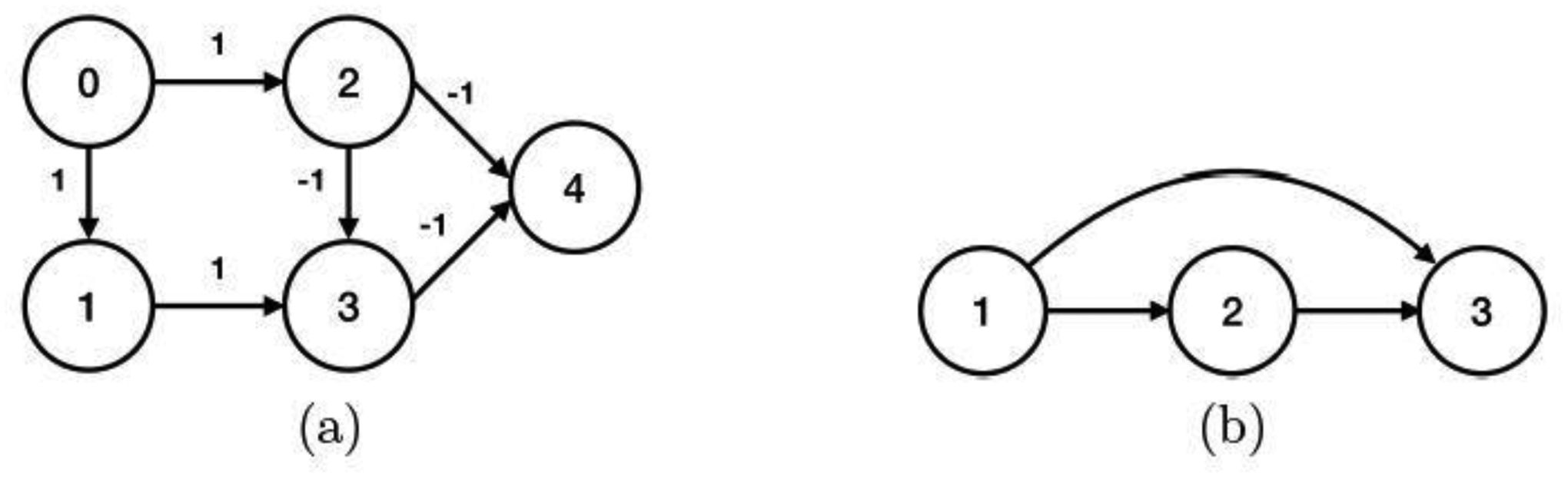
Left panel: a DAG with five nodes, where node 0 is the exposure variable, node 4 is the outcome variable, and nodes 1 to 3 are the mediators. Right panel: a DAG with three nodes.

Similarly, we can show the aggregated total effect of M₃ is zero as well. However, both M₂ and M₃ have positive and negative mediation effects, and should be viewed as significant mediators.

We conclude this section by computing the explicit number of potential paths that go through any mediator M_q. For an integer k = 2,3,…,d + 1, the total number of k-step potential paths that go through M_q, by the combinatorial theory, is $N_k(q)=\left(\begin{array}{l}d-1\hfill \\ k-2\hfill \end{array}\right)(k-1)!$. Then the total number of potential paths that go through M_q is $N(q)=\sum _{k=2}^{d+1}{N}_k(q)\ge {\mathcal{N}}_{d+1}(q)=d!$. As a result, it is highly nontrivial to test the significance of an individual mediator if we take into account all the potential paths among the mediators.

3. Test Statistics

In this section, we first consider a potential test statistic built on the power of an estimator of the coefficient matrix W₀ in model (1), and discuss its limitation. We then present our main idea, the logic of Boolean matrices, and the test statistic built on it.

3.1. Power of matrices

Matrices and vectors in this paper start the index from zero. For any matrix A, let |A| denote the matrix of the same dimension whose (i, j)th entry is |A_i,j|. We first connect the null hypothesis H₀(q₁, q₂) in (5) with the coefficient matrix W₀ in model (1). Recall that H₀(q₁, q₂) means $X_{q_1}$ is not an ancestor of $X_{q_2}$. We have the next lemma.

Lemma 1. The null H₀(q₁, q₂) holds if and only if ${\left({\left|W_0\right|}^k\right)}_{q_2,q_1}=0$ for any k = 1,…,d.

We sketch the proof of this lemma here, which is to facilitate our understanding of the problem. The key observation is that, the (q₂, q₁)th entry of |W₀|^k is the sum of the absolute values of the total effects along all k-step paths from $X_{q_1}$ to $X_{q_2}$. For instance, for k = 2,

$${\left({\left|{\mathit{W}}_0\right|}^2\right)}_{q_2,q_1}=\sum _{j=0}^{d+1}\left|W_{0,j,q_1}\right|\left|W_{0,q_2,j}\right|=\sum _{j=1}^d\left|W_{0,j,q_1}\right|\left|W_{0,q_2,j}\right|,$$

where the last equality is due to that the first row and last column of W₀ are zero vectors because of Condition (A2). If there exists a two-step path from $X_{q_1}$ to $X_{q_2}$, by definition, $W_{0,j,q_1}\ne 0$ and $W_{0,q_2,j}\ne 0$ for some j = 1,…,d, which is equivalent to ${\left({\left|W_0\right|}^2\right)}_{q_2,q_1}\ne 0$. Similarly, there exists a k-step path from X₀ to M_q if and only if ${\left({\left|W_0\right|}^k\right)}_{q_2,q_1}\ne 0$.

Let W be some consistent estimator for W₀. In view of Lemma 1, it is natural to construct a test statistic based on ${\left\{{\left(|W{|}^k\right)}_{q_2,q_1}\right\}}_{1\le k\le d}$. The major difficulty with this potential test statistic, however, is that it is unclear whether ${\left(|W{|}^k\right)}_{q_2,q_1}$ has a well tabulated limiting distribution under H₀(q₁, q₂). To better illustrate this, we first consider the case when k = 2. We have ${\left(|W{|}^2\right)}_{q_2,q_1}=\sum _{j=1}^d\left|{\widehat{W}}_{j,q_1}\right|\left|{\widehat{W}}_{q_2,j}\right|$. Under H₀(q₁, q₂) and the acyclic constraint (A1), for any j, either $W_{0,j,q_1}$ or $W_{0,q_2,j}$ equals zero. Suppose each ${\widehat{W}}_{q_1,q_2}$ is root-n consistent to $W_{0,q_1,q_2}$, and the mediator dimension d is fixed. Then we can show $\sqrt{n}{\left(|W{|}^2\right)}_{q_2,q_1}$ is asymptotically equivalent to $\sum _{1\le j\le d}\sqrt{n}\left(\left|{\widehat{W}}_{j,q_1}-W_{0,j,q_1}\right|\left|W_{0,q_2,j}\right|+\left|W_{0,j,q_1}\right|\left|{\widehat{W}}_{q_2,j}-W_{0,q_2,j}\right|\right)$. The limiting distribution, however, is not well-studied even in the fixed-d scenario. When k is large, or when the mediator dimension d diverges with the sample size n, the derivation of the asymptotic property of ${\left(|W{|}^k\right)}_{q_2,q_1}$ becomes more complicated due to the addition and multiplication operations involved in ${\left(|W{|}^k\right)}_{q_2,q_1}$. Therefore, the test statistic based on |W|^k may not be suitable for our purpose of testing significant mediators.

3.2. Logic of Boolean matrices

To overcome the difficulty regarding |W|^k, and motivated by the logic of Boolean matrices, we define a new matrix multiplication operator and a new matrix addition operator to replace the usual matrix multiplication and addition operations. Specifically, for any two real-valued matrices $A_1={\left\{a_{1,i,j}\right\}}_{ij}\in {ℝ}^{q_1\times q_2}$, $A_2={\left\{a_{2,i,j}\right\}}_{ij}\in {ℝ}^{q_2\times q_3}$, we define A₁ ⊗ A₂ to be a q₁ × q₃ matrix whose (i, j)th entry equals ${\text{max}}_{k\in \left\{1,\dots ,q_2\right\}}$ min(a_1,i,k, a_2,k,j). That is, we replace the multiplication operation in the usual matrix multiplication with the minimum operator, and replace the addition operation with the maximum operator. When A₁, A₂ are binary matrices, the minimum and maximum operators are equivalent to the logic operators “and” and “or” in Boolean algebra. The defined “⊗” operator is then equivalent to the Boolean matrix multiplication operator. Moreover, for any two real-valued matrices A₁ = {a_1,i,j}_ij, $A_2={\left\{a_{2,i,j}\right\}}_{ij}\in {ℝ}^{q_1\times q_2}$, we define A₁ ⊕ A₂ to be a q₁ × q₂ matrix whose (i, j)th entry equals max(a_1,i,j, a_2,i,j). When A₁, A₂ are binary matrices, the defined “⊕” operator is equivalent to the Boolean matrix addition operator.

Given the new definition of the multiplication and addition operators, we define $|W{|}_0^{(k)}={\left|W_0\right|}^{(k-1)}\otimes \left|W_0\right|$ in a recursive fashion, for any k ≥ 1. Next, we connect the null hypothesis H₀(q₁, q₂) in (5) with the newly defined |W₀|^(k). Its proof is given in the appendix.

Lemma 2. The null H₀(q₁, q₂) holds if and only if ${\left({\left|W_0\right|}^{(k)}\right)}_{q_2,q_1}=0$ for any k = 1,…,d.

Aggregating |W₀|^(k) for all k-step paths, k = 1,…,d, leads to the following definition,

$$W_0^{*}=\left|W_0\right|\oplus {\left|W_0\right|}^{(2)}\oplus \dots \oplus {\left|W_0\right|}^{(d)}.$$

We next define two matrices B₀ and $B_0^{*}$ that are the binary versions of W₀ and $W_0^{*}$,

$${\left(B_0\right)}_{i,j}=\left\{\begin{array}{cc}1,& \text{if }{W}_{0,i,j}\ne 0,\\ 0,& \text{otherwise },\end{array}\text{\hspace{0.17em}\hspace{0.17em}\hspace{0.17em}and\hspace{0.17em}\hspace{0.17em}\hspace{0.17em}}{B}_0^{*}=B_0\oplus B_0^{(2)}\oplus \dots \oplus B_0^{(d)}\right..$$

Then Lemma 2 immediately implies the next result.

Corollary 1. The null H₀(q₁, q₂) holds if and only if ${\left(W_0^{*}\right)}_{q_2,q_1}=0$ and ${\left(B_0^{*}\right)}_{q_2,q_1}=0$.

Corollary 1 suggests some natural test statistic for our hypotheses. Again, let W be some consistent estimator for W₀, and let W* = |W| ⊕ |W|² ⊕…⊕ |W|^d. We further define a thresholded binary version B(c) and B*(c), for a given thresholding value c, as,

$${\left\{B(c)\right\}}_{i,j}=\left\{\begin{array}{cc}1,& \text{if }\left|{\widehat{W}}_{i,j}\right|>c,\\ 0,& \text{otherwise },\end{array}\text{\hspace{0.17em}\hspace{0.17em}\hspace{0.17em}and\hspace{0.17em}\hspace{0.17em}\hspace{0.17em}}{B}^{*}(c)=B(c)\oplus B^{(2)}(c)\oplus \dots \oplus B^{(d)}(c)\right..$$ (7)

In view of Corollary 1, we expect $W_{q_2,q_1}^{*}$ to be small under H₀(q₁, q₂), and we reject H₀(q₁, q₂) when ${\left(W^{*}\right)}_{q_2,q_1}>c$ for some thresholding value c, or equivalently, when ${\left\{B^{*}(c)\right\}}_{q_2,q_1}=1$. We then build a test statistic based on W*.

Unlike the usual power of the matrix |W|^k, the limiting distribution of W* based on the logic of Boolean matrices is more tractable. Specifically, under the null hypothesis H₀(q₁, q₂), for any potential path $X_{q_1}\to X_{j_1}\to \dots \to X_{j_k}\to X_{q_2}$, such that

$${\widehat{W}}_{j_1,q_1}\ne 0,\underset{t\in \{1,\dots ,k-1\}}{\text{min}}\left|{\widehat{W}}_{j_{t+1},j_t}\right|\ne 0,\text{ and }{\widehat{W}}_{q_2,j_k}\ne 0,$$ (8)

there exist some distinct integers ℓ₁, ℓ₂ ∈{q₁, j₁,…,j_k, q₂} as functions of (q₁, {j_t}_1≤t≤k, q₂), such that $W_{0,{\ell }_2,{\ell }_1}=0$. It then follows that,

$$\begin{array}{l}\sqrt{n}{\left(W^{*}\right)}_{q_2,q_1}\le \underset{\begin{array}{c}k\in 1,\dots ,d\}\\ 1\le j_1,\dots ,j_k\le d+2\end{array}}{\text{max}}\sqrt{n}\left|{\widehat{W}}_{{\ell }_2,{\ell }_1}\right|=\underset{\begin{array}{c}k\in \left\{1,\dots ,d\right\}\\ 0\le j_1,\dots j_k\le d+1\end{array}}{\text{max}}\sqrt{n}\left|{\widehat{W}}_{{\ell }_2,{\ell }_1}-W_{0,{\ell }_2,{\ell }_1}\right|\hfill \\ \le \underset{\begin{array}{c}k\in \{1,\dots ,d\}\\ 0\le j_1,\dots ,j_k\le d+1\end{array}}{\text{max}}\underset{\begin{array}{c}0\le t\le k\\ j_0=q_1,j_{k+1}=q_2\end{array}}{\text{max}}\sqrt{n}\left|{\widehat{W}}_{j_{t+1},j_t}-W_{0,j_{t+1},j_t}\right|,\hfill \end{array}$$ (9)

where the first maximum is taken over all such k and (j₁,…,j_k) that satisfy (8). When the nonzero entries of $\sqrt{n}\left(W-W_0\right)$ are asymptotically normal, the right-hand-side of (9) converges in distribution to a maximum of some normal random variables in absolute values. Its αth upper quantile can be consistently estimated via multiplier bootstrap. This forms the basis of our proposed testing procedure.

On the other hand, the test outlined above has some limitations. One is that this test can be conservative when W₀ is highly sparse but W is not. Another limitation is that it requires the support of W to be fixed. When this fixed support condition does not hold, it would lead to an inflated type-I error rate. To address these limitations, we next develop a testing procedure that couples such a test with screening and data sample splitting to enhance its power as well as to ensure its validity.

4. Testing Procedure

In this section, we first present our full testing procedure for inference of an individual mediator. We next describe in detail some major steps of this testing procedure. Finally, we present a multiple testing procedure for simultaneous inference of multivariate mediators with a proper FDR control. Given that our test is constructed based on the LOGic of booleAN matrices, we refer our testing method as LOGAN.

4.1. The complete algorithm

Let X₁,…,X_n denote n i.i.d. copies of X, generated according to model (1). Step 1 of our testing procedure is to randomly divide the observed data into two equal halves ${\left\{X_i\right\}}_{i\in {\mathcal{I}}_1}\cup {\left\{X_i\right\}}_{i\in {\mathcal{I}}_2}$, where ${\mathcal{I}}_{\ell }$ is the set of indices of subsamples, ℓ = 1, 2. The purpose of data splitting is to ensure our test achieves a valid type-I error rate under minimal conditions when coupled with a screening step. In recent years, data splitting has been commonly used in high-dimensional estimation and inference (e.g., Chernozhukov et al., 2018; Newey and Robins, 2018; Barber and Candés, 2019; Romano and DiCiccio, 2019). One issue with data splitting is the potential loss of power due to the usage of only a fraction of data. There have been studies showing that data splitting may improve the power in some cases (Rubin et al., 2006; Romano and DiCiccio, 2019). In our setting, we construct two test statistics based on both halves of data, then combine them to derive the final decision rule. We show the test constructed this way achieves a good power both asymptotically and numerically. Moreover, one may follow the idea of Meinshausen et al. (2009) to carry out the binary split more than once, then combine the p-values from all splits. This strategy also helps mitigate the randomness the single data splitting introduces. In the regression setting, Meinshausen et al. (2009) showed empirically that this multi-split strategy improves the power than a single-split. We develop a multi-split version of our test in Section S1 of the appendix, and show its improvement in power numerically. We also note that, one may employ the multi-split strategy of Romano and DiCiccio (2019, Section 4.2.1) for power improvement. Meanwhile, these improvements all come with a price of increased computational costs.

Step 2 is to compute an initial estimator W^(ℓ) for W₀, given each half of the data ${\left\{X_i\right\}}_{i\in {\mathcal{I}}_{\ell }}$, ℓ = 1, 2. Several methods can be used here, e.g., Zheng et al. (2018); Yuan et al. (2019). We only require W^(ℓ) to be consistent to W₀.

This requirement is considerably weaker than requiring W^(ℓ) to be selection consistent; i.e., $\mathbb{I}\left({\tilde{W}}_{i,j}^{(l)}=0\right)=\mathbb{I}\left(W_{0,i,j}=0\right)$ for any i, j = 0,…,d + 1, where $\mathbb{I}(\cdot )$ is the indicator function. See Section 4.2 for more details.

Step 3 is to compute the binary matrix B^(ℓ) for B₀, given the initial estimator W^(ℓ), using (7) with c = 0. This step is straightforward, and the main purpose is to allow the subsequent decorrelated estimation step to focus only on those nonzero elements in B^(ℓ). It thus acts as a screening step, and in effect reduces the number of potential paths to a moderate level. As a benefit, it reduces the variance of the Boolean matrix-based test statistic, and increases the power of the test. See Section 4.3 for more details.

Algorithm 1.

Testing procedure for inference of an individual mediator.

Input:

The data X1,…Xn, 1 ≤ q ≤ d, and the significance level 0 < α < 1.

Step 1.

Randomly divide {1,2,…,n} into two disjoint subsets ${\mathcal{I}}_1\cup {\mathcal{I}}_2$ of equal sizes.

Step 2.

Compute an initial estimator W(ℓ) for W0, given ${\left\{X_i\right\}}_{i\in {\mathcal{I}}_{\ell }}$, ℓ= 1,2.

Step 3.

Compute the binary estimator B(ℓ) for B0, given W(ℓ), ℓ= 1,2, which is to be used for screening and also ancestor estimation in the next step.

Step 4.

Compute the decorrelated estimator W(ℓ) for W0, given W(ℓ), B(ℓ) and ${\left\{X_i\right\}}_{i\in {\mathcal{I}}_{\ell }}$, ℓ= 1,2.

(4a) Estimate the ancestors of Mq, for q = 1,…,d +1, by ACT $\left(q,W^{(\ell )}\right)=\left\{1\le j\le d:{\left\{B^{*(\ell )}\right\}}_{q,j}\ne 0\right\}$ where $B^{*(\ell )}=\left|B^{(\ell )}\right|\oplus {\left|B^{(\ell )}\right|}^{(2)}\oplus \dots \oplus {\left|B^{(\ell )}\right|}^{(d)}$.

(4b) Update the jth row of W(ℓ), for 1 ≤ j ≤ d, by fitting a penalized regression with ${\left\{X_{i,j}\right\}}_{i\in {\mathcal{I}}_{\ell }}$ being the response and ${\left\{X_{i,k}\right\}}_{i\in {\mathcal{I}}_{\mathcal{l}},{\tilde{W}}_{j,k}^{(\mathcal{l})}\ne 0}$ being the predictors. Denote the updated estimator as ${\overline{W}}^{(\ell )}$.

(4c) Compute the decorrelated estimator ${\widehat{W}}_{j_1,j_2}^{(\ell )}$, for any (j1, j2) such that ${\widehat{B}}_{j_1,j_2}^{(\ell )}\ne 0$, given ${\left\{X_i\right\}}_{i\in {\mathcal{I}}_{\ell }^c},\text{ACT}\left(j_1,W^{(\ell )}\right),B^{(\ell )}$, and ${\overline{W}}^{(\ell )}$.

Step 5.

Compute the critical values using the bootstrap procedure, given W(ℓ), B(ℓ), and ${\left\{X_i\right\}}_{i\in {\mathcal{I}}_{\ell }}$, ℓ= 1,2.

(5a) Compute the critical value ${\widehat{c}}^{(\ell )}(0,q)$ of ${\text{max}}_{(i,j)\in \mathcal{S}\left(0,q,B^{(\ell )}\right)}\sqrt{\left|{\mathcal{I}}_{\ell }^c\right|}\left|{\widehat{W}}_{i,j}^{(\ell )}-W_{0,i,j}^{(\ell )}\right|$ under the significance level α/2, ℓ= 1,2.

(5b) Compute the critical value ${\widehat{c}}^{(\ell )}(q,d+1)$ of ${\text{max}}_{(i,j)\in \mathcal{S}\left(q,d+1,B^{(\ell )}\right)}\sqrt{\left|{\mathcal{I}}_{\ell }^c\right|}\left|{\widehat{W}}_{i,j}^{(\ell )}-W_{0,i,j}^{(\ell )}\right|$ under the significance level α/2, ℓ= 1,2.

Output:

Decision.

(6a) Reject H0(0,q) if $B_{q,0}^{*(\ell )}\left\{n^{-1/2}\widehat{c}(0,q)\right\}=1$. Denote this decision by ${\mathcal{D}}^{(\ell )}(0,q)$.

(6b) Reject H0(q,d + 1) if $B_{d+1,q}^{*(\ell )}\left\{n^{-1/2}\widehat{c}(q,d+1)\right\}=1$. Denote this decision by ${\mathcal{D}}^{(\ell )}(q,d+1)$.

(6c) Reject H0(q) if both ${\mathcal{D}}^{(\ell )}(0,q)$ and ${\mathcal{D}}^{(\ell )}(q,d+1)$ reject, for at least one ℓ= 1,2.

Step 4 is to compute a decorrelated estimator W^(ℓ) using a cross-fitting procedure. We use one set of samples ${\mathcal{I}}_{\ell }$ to obtain the initial estimator W^(ℓ) and the binary version B^(ℓ) to screen out the zero entries, then use the other set of samples ${\mathcal{I}}_{\ell }^c$ to compute the entries of the decorrelated estimator W^(ℓ). This decorrelated estimation step is to reduce the bias of W^(ℓ) under the setting of high-dimensional mediators. Moreover, it guarantees the entry of W^(ℓ), ${\widehat{W}}_{j_1,j_2}^{(\ell )}$, is $\sqrt{n}$-consistent and asymptotically normal. It adopts the debiasing idea that is commonly used for statistical inference of low-dimensional parameters in high-dimensional models (Zhang and Zhang, 2014; Ning and Liu, 2017). See Section 4.3 for more details.

Step 5 is to use a bootstrap-based procedure to compute the critical values. Let

W*^(ℓ) = |W|^(ℓ) |⊕|W^(ℓ)|⁽²⁾ ⊕…⊕ |W^(ℓ)|^(d). Similar to (9), we have

$$\sqrt{\left|{\mathcal{I}}_{\ell }^c\right|}{\left(W^{*(\ell )}\right)}_{q_2,q_1}\le {\text{max}}_{\begin{array}{c}k\in \left\{1,\dots ,d\right\}\\ 0\le j_1,\dots ,j_k\le d+1\end{array}}{\text{max}}_{\begin{array}{c}0\le t\le k\\ j_0=q_1,j_{k+1}=q_2\end{array}}\sqrt{\left|{\mathcal{I}}_{\ell }^c\right|}\left|{\widehat{W}}_{j_{t+1},j_t}^{(\ell )}-W_{0,j_{t+1},j_t}^{(\ell )}\right|.$$

When ${\widehat{W}}_{j_{t+1},j_t}^{(\ell )}$ is nonzero, the mediators j_t and j_t+1 satisfy that

j_t ∈ ACT(q₂, B^(ℓ)), j_t+1 ∈ ACT(q₂, B^(ℓ)) ⋃ {q₂}, q₁ ∈ ACT(j_t, B^(ℓ)) ⋃ {j_t}, q₁ ∈ ACT(j_t+1, B^(ℓ)) and ${\widehat{B}}_{j_{t+1},j_t}^{(\ell )}=1$. Then

$$\sqrt{\left|{\mathcal{I}}_{\ell }^c\right|}{\left(W^{*(\ell )}\right)}_{q_1,q_2}\le \underset{(i,j)\in \mathcal{S}\left(q_1,q_2,{\mathit{B}}^{(\ell )}\right)}{\text{max}}\sqrt{\left|{\mathcal{I}}_{\ell }^c\right|}\left|{\widehat{W}}_{i,j}^{(\ell )}-W_{0,i,j}\right|,$$ (10)

where $\mathcal{S}\left(q_1,q_2,B^{(\ell )}\right)=\left\{(i,j):j\in \text{ACT}\left(q_2,B^{(\ell )}\right)\right.$, i ∈ ACT(q₂, B^(ℓ)) ⋃ {q₂}, q₁ ∈ ACT(j, B^(ℓ)), orj = q₁, q₁ ∈ ACT(i, B^(ℓ)), {B^(ℓ)}_i,j ≠0}. Here $\mathcal{S}\left(q_1,q_2,B^{(\ell )}\right)$ denotes the set of indices such that ${\left\{W^{*(\ell )}\right\}}_{q_1,q_2}$ depends on W^(ℓ) only through its entries in $\mathcal{S}\left(q_1,q_2,B^{(\ell )}\right)$. Then, based on (10), we use bootstrap to obtain the critical values of

$$\underset{\left(j_1,j_2\right)\in \mathcal{S}\left(0,q,{\mathit{B}}^{(\ell )}\right)}{\text{max}}\sqrt{\left|{\mathcal{I}}_{\ell }^c\right|}\left|{\widehat{W}}_{j_1,j_2}^{(\ell )}-W_{0,j_1,j_2}^{(\ell )}\right|\text{\hspace{0.17em}\hspace{0.17em}\hspace{0.17em}and\hspace{0.17em}\hspace{0.17em}\hspace{0.17em}}\underset{(j_1,j_2)\in \mathcal{S}\left(q,d+1,{\mathit{B}}^{(\ell )}\right)}{\text{max}}\sqrt{\left|{\mathcal{I}}_{\ell }^c\right|}\mid {\widehat{W}}_{j_1,j_2}^{(\ell )}-W_{0,j_1,j_2}^{(\ell )}\mid ,$$

under the significance level α / 2. Denote the two critical values by ${\widehat{c}}^{(\ell )}(0,q)$ and ${\widehat{c}}^{(\ell )}(q,d+1)$, respectively. See Section 4.4 for more details.

Once obtaining the critical values, we reject H₀(0, q) if $B_{q,0}^{*(\ell )}\left\{{\left|{\mathcal{I}}_{\ell }^c\right|}^{-1/2}{\widehat{c}}^{(\ell )}(0,q)\right\}=1$, and reject H₀(q, d + 1) if $B_{d+1,q}^{*(\ell )}\left\{{\left|{\mathcal{I}}_{\ell }^c\right|}^{-1/2}{\widehat{c}}^{(\ell )}(q,d+1)\right\}=1$. We reject the null H₀(q) when H₀(0, q) and H₀(q, d + 1) are both rejected. Note that, for each half of the data ℓ = 1, 2, we have made a decision ${\mathcal{D}}^{(\ell )}$ regarding H₀(q). Finally, we reject H₀(q). when either ${\mathcal{D}}^{(1)}$ or ${\mathcal{D}}^{(2)}$ decides to reject. By Bonferroni’s inequality, this yields a valid α-level test.

We summarize the full testing procedure in Algorithm 1.

4.2. Initial DAG estimation

There are multiple estimation methods available to produce an initial estimator for W₀, for instance, Zheng et al. (2018) and Yuan et al. (2019). We employ the method of Zheng et al. (2018) in our implementation. Specifically, we seek ${\text{min}}_{W\in {ℝ}^{(d+2)\times (d+2)}}\mathcal{L}(W)+\lambda \left|{\mathcal{I}}_{\ell }\right|\sum _{i,j}\left|W_{i,j}\right|$, subject to $\mathbb{G}(W)\in \text{DAGs }$, where $\mathcal{L}(W)=\sum _{i\in {\mathcal{I}}_{\ell }}{‖X_i-W{X}_i‖}_2^2,\lambda >0$ is a regularization parameter, $\mathbb{G}$ denotes the graph induced by W, X_i = X_i − μ is the centered covariate, $\mu =\sum _{i=1}^n{X}_i/n$, and $\left|{\mathcal{I}}_{\ell }\right|$ is the number of data samples in the data split ${\mathcal{I}}_{\ell }$. This optimization problem is challenging to solve due to the fact that the search space of DAGs scales super-exponentially with the dimension d. To resolve this issue, Zheng et al. (2018) proposed a novel characterization of the acyclic constraint, by showing that the DAG constraint can be represented by trace {exp(W^∘W)} = d + 2, where ∘ denotes the Hadamard product, exp(A) is the matrix exponential of A, and trace(A) is the trace of A. Then the problem becomes

$$\underset{{\mathit{W}\in ℝ}^{(d+2)\times (d+2)}}{\text{min}}\mathcal{L}(\mathit{W})+\lambda \left|{\mathcal{I}}_{\ell }\right|\sum _{i,j}\left|W_{i,j}\right|,\text{subject to trace }\left\{\text{exp}\left({\mathit{W}}^{\circ }\mathit{W}\right)\right\}=d+2.$$ (11)

Let W^(ℓ) denote the minimizer of (11). Zheng et al. (2018) proposed an efficient augmented Lagrangian based algorithm to solve (11). After obtaining W^(ℓ), we set the elements in its first row and last column to zero, following Condition (A2).

We make some remarks. First, the optimization in (11) is nonconvex, and there is no guarantee that the algorithm of Zheng et al. (2018) can find the global minimizer. As such, W^(ℓ) may not satisfy the acyclicity condition, although a global minimizer does. To meet the acyclicity constraint, Zheng et al. (2018) employed an additional thresholding step to truncate all the elements in the numerical solution to (11) whose absolute values are smaller than some threshold value c₀ to zero. We follow their implementation and adopt the same thresholding value c₀ = 10⁻³. Second, to achieve the theoretical guarantees of our proposed test, we only require the estimator W^(ℓ) to be a consistent estimator of W₀, which is much weaker than the requirement of the test of Chakrabortty et al. (2018) that the DAG estimator has to be selection consistent. In Section 5.2, we show that the global solution of (11) satisfies this consistency requirement (see Proposition 1). Meanwhile, as long as $c_0\ll \sqrt{n^{-1}\text{log\hspace{0.17em}}n}$, we can show Proposition 1 holds for the thresholded solution of (11) as well.

4.3. Screening and debiasing

Given the initial estimator W^(ℓ), we next compute the binary estimator B ^(ℓ) for B₀ using (7) with c = 0. We then use the nonzero entries of B^(ℓ) to determine the support of the decorrelated estimator W^(ℓ) in the subsequent step of decorrelated estimation. As such, it serves as a screening step, and allows us to reduce the number of potential paths to a moderate level. As shown in (10), the decorrelated estimator ${\left(W^{*(\ell )}\right)}_{q_1,q_2}$ depends on W^(ℓ) only through its entries in $\mathcal{S}\left(q_1,q_2,B^{(\ell )}\right)$. Consequently, the screening through B^(ℓ) reduces the variance of ${\left({\mathit{W}}^{*(\ell )}\right)}_{q_1,q_2}$, which in turn leads to an increased power for our test.

Next, we employ the decorrelated estimation idea of Ning and Liu (2017) to compute a decorrelated estimator W^(ℓ) to reduce the bias of the initial estimator W^(ℓ) obtained from (11). Because of the presence of the regularization term in (11) for high-dimensional mediators, the initial estimator W^(ℓ) may suffer from a large bias and does not have a tractable limiting distribution. To address this issue, we refit $W_{0,j_1,j_2}$ for any (j₁, j₂) such that ${\widehat{B}}_{j_1,j_2}^{(\ell )}\ne 0$, by constructing an estimating equation based on a decorrelated score function. This effectively alleviates the bias, and the resulting decorrelated estimator ${\widehat{W}}_{j_1,j_2}^{(\ell )}$ is both $\sqrt{n}$-consistent and asymptotically normal.

More specifically, after some calculations, we have that,

$$\begin{gathered} \text{E}\left(X_{j_1}-\sum _{j\ne j_2}{W}_{0,j_1,j}{X}_j\right)\left(X_{j_2}-\text{E}\left[X_{j_2}\mid {\left\{X_j\right\}}_{j\in \text{ACT}\left(j_2,W_0\right)}\right]\right) \\ =W_{0,j_1,j_2}\text{E}\left\{X_{j_2}\left(X_{j_2}-\text{E}\left[X_{j_2}\mid {\left\{X_j\right\}}_{j\in \text{ACT}\left(j_2,W_0\right)}\right]\right)\right\}, \end{gathered}$$ (12)

which is the estimating equation to construct our decorrelated estimator ${\widehat{W}}_{0,j_1,j_2}$ . Toward that end, we need to estimate $\text{E}\left[X_{j_2}\mid {\left\{X_j\right\}}_{j\in \text{ACT}\left(j_2,W_0\right)}\right]$ and $\left\{W_{0,j_1,j}:j\ne j_2\right\}$.

To estimate $\text{E}\left[X_{j_2}\mid {\left\{X_j\right\}}_{j\in \text{ACT}\left(j_2,W_0\right)}\right]$, we first estimate the set of ancestors of the j₂th node ACT(j₂, W₀) by $\text{ACT}\left(j_2,W^{(\ell )}\right)=\left\{1\le j\le d:{\left(W^{*(\ell )}\right)}_{j_2,j}\ne 0\right\}$, for j₂ = 1,…,d + 1, where W*^(ℓ) =|W^(ℓ)|⊕|W^(ℓ)|⁽²⁾ ⊕…⊕|W^(ℓ)|^(d). We also note that, when estimating the ancestors, we always include the exposure variable E = X₀ in the set of ancestors, and always include all mediators when estimating the ancestors of the outcome variable Y = X_d+1. Next, we approximate $\text{E}\left[X_{j_2}\mid {\left\{X_j\right\}}_{j\in \text{ACT}\left(j_2,W^{(\ell )}\right)}\right]$ using a linear regression model, where the regression coefficients are estimated by,

$${\beta }_{j_1,j_2}^{(\ell )}=\underset{\begin{array}{c}\beta :{\beta }_{j_2}=0\\ \text{supp}(\beta )\in \text{ACT}\left(j_1,W^{(\ell )}\right)\end{array}}{\text{argmin}}\left\{\frac{1}{\left|{\mathcal{I}}_{\ell }^c\right|}\sum _{i\in {\mathcal{I}}_{\ell }^c}{\left({\tilde{X}}_{i,j_2}-{\beta }^{\top }{X}_i\right)}^2+\sum _{\begin{array}{c}k:k\ne j_2,\\ k\in \text{ACT}\left(j_1,{\mathit{W}}^{(\ell )}\right)\end{array}}{p}_{\lambda }\left(\left|{\beta }_k\right|\right)\right\},$$ (13)

where supp(β) denotes the support of $\mathit{\beta }\in {ℝ}^{d+2}$, and the regression fitting is done based on the complement set of samples ${\mathcal{I}}_{\ell }^c$. We choose the MCP (Zhang, 2010) penalty function and tune the penalty parameter by the Bayesian information criterion in our implementation. Alternatively, we can use LASSO (Tibshirani, 1996), SCAD (Fan and Li, 2001) or Dantzig selector (Candes and Tao, 2007) in (13). It is crucial to note that, the resulting estimator is $\sqrt{n}$-consistent regardless of whether the linear model approximation holds or not.

To estimate $\left\{W_{0,j_1,j}:j\ne j_2\right\}$, we employ a refined version of the initial estimator W^(ℓ). That is, we update the jth row of W^(ℓ), j = 1,…,d, by fitting a penalized regression with ${\left\{X_{i,j}\right\}}_{i\in {\mathcal{I}}_{\ell }}$ being the response and ${\left\{X_{i,k}\right\}}_{i\in {\mathcal{I}}_{\ell },{\tilde{W}}_{j,k}^{(\ell )}\ne 0}$ being the predictors. We again use the MCP penalty. Denote the resulting refined estimator by ${\overline{\mathit{W}}}^{(\ell )}$. The purpose of this refitting is to improve the estimation efficiency of the initial estimator W^(ℓ). In our numerical experiments, we find ${\overline{\mathit{W}}}^{(\ell )}$ usually converges faster than W^(ℓ) to the truth.

Built on the above estimators and the estimating equation (12), we debias ${\tilde{W}}_{j_1,j_2}^{(\ell )}$ using the other half of the data ${\left\{X_i\right\}}_{i\in {\mathcal{I}}_{\ell }^c}$, for any entry such that ${\widehat{B}}_{j_1,j_2}^{(\ell )}\ne 0$, by

$${\widehat{W}}_{j_1,j_2}^{(\ell )}=\frac{\sum _{i\in {\mathcal{I}}_{\ell }^c}\left({\tilde{X}}_{i,j_2}-{\beta }_{j_1,j_2}^{(\ell )\top }{X}_i\right)\left({\tilde{X}}_{i,j_1}-\sum _{j\ne j_2}{\tilde{X}}_{i,j}{\overline{W}}_{j_1,j}^{(\ell )}\right)}{\sum _{i\in {\mathcal{I}}_{\ell }^c}{\tilde{X}}_{i,j_2}\left({\tilde{X}}_{i,j_2}-{\beta }_{j_1,j_2}^{(\ell )}{X}_i\right)}.$$ (14)

We remark that, we have used the cross-fitting strategy in both the estimation of ${\beta }_{j_1,j_2}^{(\ell )}$ in (13), and in the decorrelated estimation of ${\widehat{W}}_{j_1,j_2}^{(\ell )}$ in (14). This strategy guarantees each entry of the decorrelated estimator W^(ℓ) is asymptotically normal, regardless of whether the initial estimator W^(ℓ) is selection consistent or not.

4.4. Bootstrap for critical values

We next develop a multiplier bootstrap method to obtain the critical values, and summarize this procedure in Algorithm 2. Our goal is to approximate the limiting distribution of ${\widehat{S}}^{(\ell )}={\text{max}}_{\left(j_1,j_2\right)\in \mathcal{S}\left(q_1,q_2,B^{(\ell )}\right)}\sqrt{\left|{\mathcal{I}}_{\ell }^c\right|}\left|{\widehat{W}}_{j_1,j_2}^{(\ell )}-W_{0,j_1,j_2}\right|$ on the right-hand-side of (10).

We first observe that $\sqrt{\left|{\mathcal{I}}_{\ell }^c\right|}\left({\widehat{W}}_{j_1,j_2}^{(\ell )}-W_{0,j_1,j_2}\right)$ is asymptotically equivalent to

$${\eta }_{j_1,j_2}^{(\ell )}=\frac{\sqrt{\left|{\mathcal{I}}_{\ell }^c\right|}\mid \sum _{i\in {\mathcal{I}}_{\ell }^c}\left\{{\tilde{X}}_{i,j_2}-{\beta }^{(\ell )\top }\left(j_1,j_2\right)X_i\right\}{\epsilon }_{i,j_1}}{\sum _{i\in {\mathcal{I}}_{\ell }^c}{\tilde{X}}_{i,j_2}\left\{{\tilde{X}}_{i,j_2}-{\beta }^{(\ell )\top }\left(j_1,j_2\right)X_i\right\}}.$$ (15)

Correspondingly, ${\widehat{S}}^{(\ell )}={\text{max}}_{\left(j_1,j_2\right)\in \mathcal{S}\left(q_1,q_2,B^{(\ell )}\right)}\left|{\eta }_{j_1,j_2}^{(\ell )}\right|+o_p(1)$, for any q₁ ∈{0,1…,d} and q₂ ∈{1,…,d + 1}. Conditioning on $\left\{X_{i,j}:i\in {\mathcal{I}}_{\ell }^c,j\in \text{ACT}\left(j_1,W^{(\ell )}\right)\right\}$, ${\eta }_{j_1,j_2}^{(\ell )}$ corresponds to a sum of independent mean zero random variables, and is asymptotically normal. A rigorous proof is given in Step 1 of the proof of Theorem 1 in the appendix. This implies that $\sqrt{\left|{\mathcal{I}}_{\ell }^c\right|}\left({\widehat{W}}_{j_1,j_2}^{(\ell )}-W_{0,j_1,j_2}\right)$ is asymptotically normal. Therefore, ${\widehat{S}}^{(\ell )}$ is to converge in distribution to a maximum of normal random variables in absolute values. Its quantile can be consistently estimated by a multiplier bootstrap method (Chernozhukov et al., 2013).

Algorithm 2.

Bootstrap procedure to obtain the critical values.

Input:

The data $\left\{X_i:i\in {\mathcal{I}}_{\ell }^{(c)}\right\}$, the significance level α, the variance estimator ${\widehat{\sigma }}_{*}^2$, the number of bootstrap samples m, the estimator ${\beta }^{(\ell )}\left(j_1,j_2\right)$ from (13), and the set $\mathcal{S}\left(q_1,q_2,B^{\left(\ell \right)}\right)$.

Step 1.

Generate i.i.d. standard normal random variables ${\left\{e_{i,j}^{(b)}\right\}}_{i,j},b=1,2,\dots ,m$.

Step 2.

Compute ${\eta }_{j_1,j_2}^{{(\ell ,b)}^{*}}$ according to (16), with $e_{i,j_1}$ replaced by $e_{i,j_1}^{(b)}$ and $T^{(\ell ,b)}\left(q_1,q_2\right)=\underset{\left(j_1,j_2\right)\in s\left(q_1,q_2,B^{(\ell )}\right)}{\text{max}}\left|{\eta }_{j_1,j_2}^{{(\ell ,b)}^{*}}\right|,b=1,2,\dots ,m$.

Output:

The empirical upper ath quantile of $\left\{T^{(\ell ,b)}\left(q_1,q_2\right):b=1,\dots ,m\right\}$.

More specifically, one can generate the bootstrap samples by replacing the residual term ${\sigma }_{*}^{-1}\left({\tilde{X}}_{i,j_1}-\sum _i{\tilde{X}}_{i,j}{\tilde{W}}_{i,j}^{(\ell )}\right)$ in (14) with i.i.d. standard normal noise {e_i,j :1 ≤ i ≤ n, 0 ≤ j ≤ d + 1} that are independent of the data. That is, we approximate ${\eta }_{j_1,j_2}^{(\ell )}$ in (15) by

$${\eta }_{j_1,j_2}^{*(\ell )}=\frac{\sqrt{\left|{\mathcal{I}}_{\ell }^c\right|}\sum _{i\in {\mathcal{T}}_{\ell }^c}\left\{{\tilde{X}}_{i,j_2}-{\beta }^{(\ell )\top }\left(j_1,j_2\right)X_i\right\}{e}_{i,j_1}{\widehat{\sigma }}_{*}}{\sum _{i\in {\mathcal{I}}_{\ell }^c}{\tilde{X}}_{i,j_2}\left\{{\tilde{X}}_{i,j_2}-{\beta }^{(\ell )\top }\left(j_1,j_2\right)X_i\right\}},$$ (16)

where ${\widehat{\sigma }}_{*}$ is some consistent estimator of σ_*. We propose to estimate ${\sigma }_{*}^2$ by ${\widehat{\sigma }}_{*}^2={\left\{n(d+2)\right\}}^{-1}\sum _{\ell \in \left\{1,2\right\}}\sum _{i\in {\mathcal{I}}_i^c}\sum _{j=0}^{d+1}{\left|{\tilde{X}}_{i,j}-{\overline{W}}_j^{(\ell )\top }{X}_i\right|}_2^2$, where ${\overline{W}}_j^{(\ell )}$ denotes the jth row of ${\overline{W}}^{(\ell )}$. This estimation utilizes sample splitting again, which alleviates potential bias of the variance estimator resulting from the high correlations between the noises and the mediators in the high-dimensional setting (Fan and Lv, 2008). Lemma 4 in Section S4 of the appendix shows that ${\widehat{\sigma }}_{*}^2$ is indeed consistent. Then the limiting distribution of ${\widehat{S}}^{(\ell )}$ can be well approximated by the conditional distribution of the bootstrap samples given the data. A formal justification is given in Step 3 of the proof of Theorem 1 in the appendix.

4.5. False discovery rate control

We next present a multiple testing procedure for simultaneous inference of multivariate mediators with a proper FDR control. We present the full procedure in Algorithm 3, which consists of four steps. We next detail each step. Let $\mathcal{N}$ be the set of unimportant mediators and $\mathcal{H}$ be the set of our selected mediators. The FDR is defined as the expected proportion of falsely selected mediators, i.e., $\text{FDR}(\mathcal{H})=\text{E}\{|\mathcal{N}\cup \mathcal{H}|/\text{max}(1,|\mathcal{H}|)\}$.

First, we compute the p-value of testing H₀(q₁, q₂), q₁ = 0,…,d, q₂ = 1,…,d + 1, for each half of the data. Specifically, we compute the decorrelated estimator W^(ℓ) in Step 4 of Algorithm 1, and W*^(ℓ) =|W^(ℓ)|⊕|W^(ℓ)|⁽²⁾ ⊕…⊕ |W^(ℓ)|^(d). We next compute T^(ℓ,b)(q₁, q₂), b = 1,…,m, in Step 2 of Algorithm 2. Then the p-value of testing H₀(q₁, q₂) in (5) is

$${\widehat{p}}^{(\ell )}\left(q_1,q_2\right)=\frac{1}{m}\sum _{b=1}^m\mathbb{I}\left\{T^{(\ell ,b)}\left(q_1,q_2\right)\ge \sqrt{{\mathcal{I}}_{\ell }^c}{\left({\mathit{W}}^{*(\ell )}\right)}_{q_2,q_1}\right\}.$$ (17)

The p-values of testing H₀(0, q) and H₀(q, d + 1) are ${\widehat{p}}^{(\ell )}(0,q)$ and ${\widehat{p}}^{(\ell )}(q,d+1)$, respectively.

Algorithm 3.

Multiple testing procedure for inference of multivariate mediators.

Input:

The significance level α, and the thresholding values 0 < c(1), c(2) < 1.

Step 1.

Compute the p-values of testing the null hypothesis H0 (q1, q2) for q1 = 0,…,d, q2 = l,…,d + l using (17) for each half of the data, ℓ = 1,2.

Step 2.

Screening based on the pairwise minimum p-values, ${\widehat{p}}_{\text{min}}^{(\ell )}(q)=\text{min}\left\{{\widehat{p}}^{(\ell )}(0,q),{\widehat{p}}^{(\ell )}(q,d+1)\right\}$. Let ${\mathcal{H}}_0^{(\ell )}=\left\{1\le q\le d:{\widehat{p}}_{\text{min}}^{(\ell )}(q)\le c^{(\ell )}\right\}$ denote the set of the initially selected mediators, ℓ = 1,2.

Step 3.

Order by the pairwise maximum p-values, ${\widehat{p}}_{\text{max}}^{(\ell )}(q)=\text{max}\left\{{\widehat{p}}^{(\ell )}(0,q),{\widehat{p}}^{(\ell )}(q,d+1)\right\}$, for those mediators in ${\mathcal{H}}_0^{(\ell )}$, as ${\widehat{p}}_{(1)}^{(\ell )}\le {\widehat{p}}_{(2)}^{(\ell )}\le \dots \le {\widehat{p}}_{\left(\left|H_0^{(\ell )}\right|\right)}^{(\ell )}$.

Step 4.

Select $h^{(\ell )}$ mediators in ${\mathcal{H}}_0^{(l)}$ with the smallest p-values. Let ${\mathcal{H}}^{(\ell )}$ denote the set of selected mediators, ℓ = 1,2.

Output:

$\mathcal{H}={\mathcal{H}}^{(1)}\cup {\mathcal{H}}^{(2)}$.

Next, we adopt and extend the ScreenMin procedure proposed by Djordjilović et al. (2019) to our setting. We begin by computing the pairwise minimum p-values, ${\widehat{p}}_{\text{min}}^{(\ell )}(q)=\text{min}\left\{{\widehat{p}}^{(\ell )}(0,q),{\widehat{p}}^{(\ell )}(q,d+1)\right\}$. We then screen and select those mediators whose corresponding ${\widehat{p}}_{\text{min}}^{(\ell )}(q)$ is smaller than a thresholding value c^(ℓ), which is determined adaptively by $c^{(\ell )}=\text{max}\left\{c\in (\alpha /d,\dots ,\alpha /2,\alpha ):c\left|{\mathcal{H}}_0^{(\ell )}(c)\right|\le \alpha \right\}$, and ${\mathcal{H}}_0^{(\ell )}(c)$ denotes the set of prescreened mediators when the threshold value is c. Djordjilović et al. (2019) showed such a thresholding value approximately maximizes the power to reject false union hypotheses. It also works well in our numerical studies. Denote the resulting set of important mediators by the ScreenMin procedure as ${\mathcal{H}}_0^{(\ell )}$.

Next, we compute the pairwise maximum p-value, which is also the p-value of testing the significance of an individual mediator H₀(q) in our setting, ${\widehat{p}}_{\text{max}}^{(\ell )}(q)=\text{max}\left\{{\widehat{p}}^{(\ell )}(0,q),{\widehat{p}}^{(\ell )}(q,d+1)\right\}$. We order the mediators in ${\mathcal{H}}_0^{(\ell )}$ according to ${\widehat{p}}_{\text{max}}^{(\ell )}(q)$.

Finally, we apply the procedure of Benjamini and Yekutieli (2001) to the ordered mediators, and select h^(ℓ) mediators with the smallest p-values, where $h^{(\ell )}=\text{max}\left[i:{\widehat{p}}_{(i)}^{(\ell )}\le (i\alpha )/\left\{2\left|{\mathcal{H}}_0^{(\ell )}\right|\sum _{j=1}^{\left|{\mathcal{H}}_0^{(\ell )}\right|}{j}^{-1}\right\}\right]$. Letting ${\mathcal{H}}^{(\ell )}$ denote the selected mediators for each half of the data, ℓ = 1, 2, respectively, we set the final set of selected mediators as $\mathcal{H}={\mathcal{H}}^{(1)}\cup {\mathcal{H}}^{(2)}$.

5. Theory

In this section, we first establish the consistency of our test for each individual mediator, by deriving the asymptotic size and power. We then show that the multiple testing procedure achieves a valid FDR control. Finally, as a by-product, we derive an oracle inequality for the estimator W^(ℓ) computed from (11) using the method of Zheng et al. (2018).

5.1. Consistency and FDR control

We first present a main regularity condition (A4), while we defer two additional regularity conditions (A5) and (A6) to Section S3 of the appendix in the interest of space.

1. With probability approaching one, ACT (j, W^(ℓ)) contains all parents of j, for any j = 0, …,d +1, ℓ = 1, 2.

This condition requires an appropriate identification of the graph, in that ACT (j, W^(ℓ)) contains all parents of j. It serves as a basis for the asymptotic properties of the proposed test. We make some remarks. First, this condition is weaker than requiring ${\mathit{W}}_j^{(\ell )}$, the jth column of W^(ℓ) , to satisfy the sure screening property; i.e, $\text{PA}(j)\subseteq \text{supp}\left(W_j^{(\ell )}\right)$, where PA(j) denotes the parents of node j. To better illustrate this, consider the DAG example in Figure 1(b). For node j = 3, the sure screening property of $W_3^{(\ell )}$ requires W_0,3,1 and W_0,3,2 to satisfy certain minimum-signal-strength conditions; see, e.g., Fan and Lv (2008). In comparison, we require {1, 2} ∈ ACT(3, W^(ℓ)) with probability approaching one. This requires either {W_0,3,1, W_0,3,2}, or {W_0,2,1, W_0,3,2} , to satisfy certain minimum-signal-strength conditions. In that sense, our test is “doubly robust”. In Proposition 1, we show (A4) is satisfied when the initial estimator is obtained using (11) of Zheng et al. (2018). Second, we remark that, when (A4) is not satisfied, the bias in the ancestor identification step is to affect the subsequent testing procedure. This phenomenon is similar to post-selection inference in linear regressions, where direct inference may fail when the variable selection step does not satisfy the sure screening or selection consistency property (Meinshausen et al., 2009; Shi et al., 2019; Zhu et al., 2020). In the linear regression setting, debiasing is an effective remedy to address the issue. However, the usual debiasing strategy may not be directly applicable in our setting; see Section S3 of the appendix for more discussion. We leave this post-selection inference problem as future research.

We next establish the validity of our test for a single mediator in Theorem 1, and its local power property in Theorem 2. Combining the two theorems yields its consistency.

Theorem 1. Suppose (A1) to (A5) hold. Suppose $d=O\left(n^{{\kappa }_1}\right)$ for some constant κ₁ > 0, and ‖W₀‖₂ is bounded. Then for a significance level 0 < α < 1, and any mediator q = 1,…,d, the proposed test in Algorithm 1 satisfies that

$$\text{Pr}\left\{H_0(q)\text{ is rejected }|H_0(q)\text{ holds }\right\}\le \alpha +o(1).$$

Next, for any directed path $\zeta :E\to M_{i_1}\to \dots \to M_{i_k}\to Y$, define ${\omega }_{\xi }^{*}$ as the minimum signal strength along this path,

$${\omega }_{\zeta }^{*}=\text{min}\left\{\left|W_{0,i_1,0}\right|,\underset{j\in \left\{1,k-1\right\}}{\text{min}}\left|W_{0,i_{j+1}{i}_j}\right|,\left|W_{0,d+1,i_k}\right|\right\}.$$

Under the alternative hypothesis H₁(q), there exists at least one path ζ that passes through M_q such that ${\omega }_{\zeta }^{*}>0$. We next establish the local power property of our test.

Theorem 2. Suppose the conditions in Theorem 1 hold. Suppose ${\text{max}}_{j\in \left\{0,1,\dots ,d+1\right\}}{‖W_j^{(\ell )}-W_{0,j}‖}_2=O_p\left(n^{-1/2}\sqrt{\text{log\hspace{0.17em}}n}\right)$, where $W_j^{(\ell )}$ is the jth row of W_j.

Suppose there exists one path $\zeta :E\to M_{i_1}\to \dots \to M_{i_k}\to Y$ that passes through M_q such that ${\omega }_{\zeta }^{*}\gg n^{-1/2}\sqrt{\text{log\hspace{0.17em}}n}$ under H₁(q). Then the proposed test in Algorithm 1 satisfies that,

$$\text{Pr}\left\{H_0(q)\text{ is rejected }|H_1(q)\text{ holds }\right\}\to 1,\text{ as }n\to \infty .$$

Note that we require ${\omega }_{\xi }^{*}\gg n^{-1/2}\sqrt{\text{log\hspace{0.17em}}n}$ for some ζ in Theorem 2. Consequently, our test is consistent against some local alternatives that are $\sqrt{n}$-consistent to the null up to some logarithmic term. Let s₀ = max_j | supp(W_0,j) | denotes the maximum sparsity size where W_0,j stands for the jth row of W₀. In Proposition 1, we show that ${\text{max}}_{j\in \{0,\dots ,d+1\}}{‖W_j^{(\ell )}-W_j‖}_2=O_p\left(n^{-1/2}\sqrt{\text{log\hspace{0.17em}}n}\right)$ when the maximum sparsity size s₀ is bounded.

Next, we show that our multiple testing procedure achieves a valid FDR control. Note that we use a union-intersection principle to construct the p-value for H₀(q). The key idea of the ScreenMin procedure of Djordjilović et al. (2019) lies in exploiting the independence between the two p-values ${\widehat{p}}^{(\ell )}(0,q)$ and ${\widehat{p}}^{(\ell )}(q,d+1)$. In our setting, these p-values are actually asymptotically independent. We thus have the following result.

Theorem 3. Suppose the conditions in Theorem 1 hold. Then the set of selected mediators $\mathcal{H}$ in Algorithm 3 satisfies that $\text{FDR}(\mathcal{H})\le \alpha +o(1)$.

5.2. Oracle inequality for the initial DAG estimator

As a by-product, we establish the oracle inequality for the estimator of Zheng et al. (2018). We first introduce the oracle estimator. For a given ordering π = {π₀, π₁,…,π_d+1}, consider the estimator

$$\begin{gathered} W^{(\ell )}(\pi )={\left\{W_0^{(\ell )}(\pi ),W_1^{(\ell )}(\pi ),\dots ,W_{d+1}^{(\ell )}(\pi )\right\}}^{\top }\text{ where } \\ {W}_{{\pi }_j}^{(\ell )}(\pi )=\underset{\beta :\text{supp}(\beta )\in \left\{{\pi }_0,{\pi }_1,\dots ,{\pi }_{j-1}\right\}}{\text{argmin}}\sum _{i\in {\mathcal{I}}_{\ell }}{\left(X_{i,{\pi }_j}-{\beta }^{\top }{X}_i\right)}^2+\lambda \left|{\mathcal{I}}_{\ell }\right|\parallel \beta {\parallel }_1, \end{gathered}$$

for j ∈ {0, 1, …,d +1}. That is, W^(ℓ) (π) is computed as if the ordering of π were known. Let Π* denote the set of all true orderings, while a more rigorous definition is given in Section S3 of the supplementary appendix. Then the oracle estimator $W_{{\pi }_j}^{(\ell )}\left({\pi }^{*}\right)$, for some π* ∈Π*, is computed as if the true ordering π* were known. With a proper choice of λ, it follows from the oracle inequality for LASSO (Bickel et al., 2009) that,

$$\underset{j\in \left\{0,\dots ,d+1\right\}}{\text{max}}{‖W_j^{(\ell )}\left({\pi }^{*}\right)-W_{0,j}‖}_2\le O(1)n^{-1/2}\sqrt{s_0\text{log\hspace{0.17em}}n}.$$

The next proposition establishes the convergence rate of W^(ℓ) obtained from (11).

Proposition 1. Suppose (A1), (A2), (A3) and (A6) hold. Suppose $d=O\left(n^{{\kappa }_1}\right)$ for some constant κ₁ < 1, ‖W₀‖₂ is bounded, and $\lambda ={\kappa }_2{n}^{-1/2}\sqrt{\text{log\hspace{0.17em}}n}$ for some sufficiently large constant κ₂ > 0. Then with probability tending to 1, the initial estimator W^(ℓ) obtained from (11) satisfies that,

$$W^{(\ell )}=W^{(\ell )}\left({\pi }^{*}\right)\text{ for some }{\pi }^{*}\in {\Pi }^{*},\text{ and }\underset{j\in (0,\dots d+1)}{\text{max}}{‖W_j^{(\ell )}-W_{0,j}‖}_2\le O(1)n^{-1/2}\sqrt{s_0\text{log\hspace{0.17em}}n}.$$

Proposition 1 shows that the convergence rate of W^(ℓ) is the same as that of the oracle estimator. Moreover, the true ordering π* can be inferred from W^(ℓ). If we produce the initial estimator from (11), it further implies that (A4) holds. We again make some remarks. First, in this proposition, we require the dimension d to grow at a slower rate than n. We note that this condition is not needed in Theorems 1–3. Moreover, we can further relax this requirement on d by imposing some sparsity conditions on W^(ℓ) and the population limit of W^(ℓ)(π); see the final remark of the proof of Proposition 1 in the appendix. Second, this proposition is for the global minimizer of (11). Of course, as we have commented, there is no guarantee that the algorithm of Zheng et al. (2018) can find the global minimizer. This is a universal problem for almost all nonconvex optimizations. Nevertheless, Zhong et al. (2014, Theorem 1) showed that the actually minimizer to (11), which is obtained through the proximal quasi-Newton method, converges to the local minimizer of the augmented Lagrange problem, while Zheng et al. (2018, Table 1) showed that numerically the difference between the actual minimizer and the global minimizer is much smaller than that between the global minimizer and the ground truth. As such, we expect Proposition 1 to hold for the actually minimizer as well. Meanwhile, we acknowledge that this local minimizer problem is challenging and is warranted for future research.

Table 1.

Identified significant mediators for the amyloid positive and amyloid negative groups.

Amyloid positive group	Amyloid negative group
r-entorhinal	l-entorhinal	l-precuneus	l-superiortemporal
	r-inferiorparietal	r-superiorfrontal	r-superiortemporal

6. Simulations

We simulate the data following model (1). We set μ₀ to a vector of ones, and ${\sigma }_{*}^2=1$. We generate the adjacency matrix W₀ as follows: We begin with a zero matrix, then replace every entry $W_{0,j_1,j_2}$ in the lower off-diagonals by the product of two random variables $R_{j_1,j_2}^{(1)}{R}_{j_1,j_2}^{(2)}$. Here $R_{j_1,j_2}^{(1)}~\text{Bernoulli}\left(p_1\right)$, if j₂ = 0, or j₁ = d + 1, and $R_{j_1,j_2}^{(1)}~\text{Bernoulli}\left(p_2\right)$, otherwise, and $R_{j_1,j_2}^{(2)}$ is uniformly distributed on [−2, −0.5]⋃[0.5, 2]. All these variables are independently generated. We consider three scenarios of the total number of mediators d, with varying binary probabilities p₁, p₂, each under two sample sizes n; i.e., (d, p₁, p₂) = (50, 0.05, 0.15) with n = 100, 200, (d, p₁, p₂) = (100, 0.03, 0.1) with n = 250, 500, and (d, p₁, p₂) = (150, 0.02, 0.05) with n = 250, 500. Table S1 in Section S10 of the appendix reports the corresponding mediators with nonzero mediation effects, and their associated δ(q), where $\delta (q)={\left(W_0^{*}\right)}_{d+1,q}{\left(W_0^{*}\right)}_{q,0}$, and $W_0^{*}$ is constructed based on W₀, q = 1,…,d. By Lemma 2, δ(q) measures the size of the mediation effect. When δ(q) = 0, H₀(q) holds; otherwise, H₁(q) holds. A larger δ(q) indicates a stronger mediation effect. The percentage of nonzero mediators for the three scenarios is 0.12, 0.09 and 0.06, respectively.

We first evaluate the empirical performance of our test for a single mediator in Algorithm 1. We also compare it with that of Chakrabortty et al. (2018), which they named as Mediation Interventional calculus when the DAG is Absent (MIDA). We use the same initial estimator as ours for MIDA. We construct the 100(1−α)% confidence interval for the total effect of each mediator, following the procedure as described in Chakrabortty et al. (2018). We reject the null hypothesis if zero is not covered by the confidence interval.

We evaluate each testing method by the empirical rejection rate, in percentage, out of 500 data replications at the significance level α = 5%. This rate reflects the size of the test when the null hypothesis holds, and reflects the power otherwise. We also compute the average receiver operating characteristic (ROC) curves, aggregated over 500 replications, when the significance level α varies. Figure 2 reports the results when d = 50. The results for d = 100 and d = 150 show a similar qualitative pattern, and are reported in Section S10 of the appendix. We make a few observations. First, our test achieves a valid size under the null hypothesis. The empirical rejection rate is close to or below the nominal level for most cases. When the sample size n is small, our test has a few inflated type-I errors. As n increases, all the rejection rates are below the nominal level. By contrast, the test of Chakrabortty et al. (2018) still has a good number of inflated type-I errors even when n is large. Such inflated errors may be due to the fact that MIDA relies on the selection consistency of the estimated DAG, which may not hold under the finite samples. Second, our test consistently achieves a larger empirical power over MIDA under the alternative hypothesis. This may be due to that the effects calculated by MIDA along different paths may cancel each other, leading to a decreased power. Combined with the results on the empirical size, the power of our test is not gained at the cost of the inflated Type-I errors. Moreover, the empirical power of our test increases along with the sample size, demonstrating the consistency of the test. Finally, we observe that the ROC curve of our test lies above that of MIDA in all settings as α varies, which clearly demonstrates the advantage of our test over MIDA.

Fig. 2.

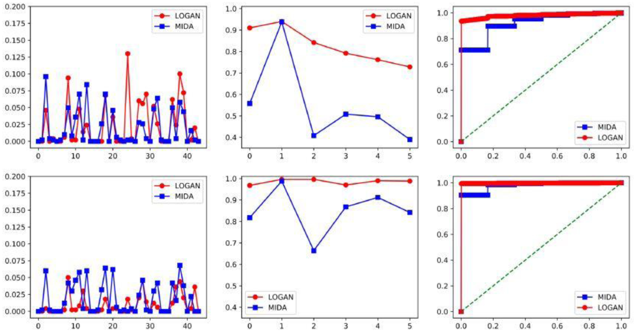
Empirical rejection rate and ROC curve of the proposed test, LOGAN, and the test of Chakrabortty et al. (2018), MIDA, when d = 50. The upper panels: n = 100, and the bottom panels: n = 200. The left panels: under H₀, the middles panels: under H₁, where the horizontal axis is the mediator index, and the right panels: the average ROC curve.

We next evaluate the empirical performance of our multiple testing procedure in Algorithm 3. We also compare it with the standard Benjamini-Yekutieli (BY) procedure. For the latter, in Step 2 of Algorithm 3, instead of applying ScreenMin to determine the set ${\mathcal{H}}_0^{(\ell )}$, one simply sets ${\mathcal{H}}_0^{(\ell )}=\left\{1,2,\dots ,d\right\}$, i.e., the set of all mediators. We evaluate each testing procedure by the false discovery rate (FDR) and the true positive rate (TPR), over 500 data replications. Figure 3 reports the results under the varying significance level α from 0 to 0.4 when d = 50. The results for d = 100 and d = 150 are similar, and are reported in Section S10 of the appendix. It is seen that both methods achieve a valid false discovery control, in that the FDRs are all below the nominal level. However, our method is more powerful than BY, as reflected by a larger TPR in all cases.

Fig. 3.

False discover rate and true positive rate of the proposed method and the Benjamini-Yekutieli procedure when d = 50. The horizontal axis corresponds to the significance level α. The left two panels: n = 100, and the right two panels: n = 200.

7. Application

In this section, we illustrate our testing method with an application to a neuroimaging study of Alzheimer’s disease (AD). AD is an irreversible neurodegenerative disorder, and is characterized by progressive impairment of cognitive and memory functions. It is the leading form of dementia, and the sixth leading cause of death in the U.S (Alzheimer’s Association, 2020). The data we analyze is part of the ongoing Berkeley Aging Cohort Study. It consists of 698 participants aging between 55.3 and 94.1 years old. For each participant, the well established PACC composite score was recorded, which combines tests that assess episodic memory, timed executive function, and global cognition (Donohue et al., 2014). Moreover, for each participant, a 1.5T structural magnetic resonance imaging (MRI) scan and a positron emission tomography (PET) scan using 18-F florbetaben tracer were acquired. All imaging data were preprocessed following the established protocols. Particularly, for MRI, all T1 images were bias-corrected, segmented, then warped and normalized to a common template space. Then the volumes were examined quantitatively by a cortical surface-based analysis and turned into cortical thickness measures. Cortical thickness is an important biomarker that reflects AD severity. We employ the FreeSurfer brain atlas and summarize each MRI image by a 68-dimensional vector, whose entries measure cortical thickness of 68 brain regions of interest. For PET, native-space images were realigned and coregistered to each participant’s MRI scan, and centiloid analysis was performed to transform the standardized uptake value ratio to centiloid units. The PET scan provides a measure of deposition of amyloid-beta, a hallmark pathological protein of AD that is commonly found in the brains of AD and elderly subjecs. The total amount of amyloid-beta deposition was extracted from PET for each subject. There are well validated methods for thresholding the subjects based on the total deposition as amyloid positive and amyloid negative groups, which are known to behave differently in AD progression (Landau et al., 2013). For our data, 309 subjects were classified as amyloid positive, and 389 as amyloid negative. Since age is a well known risk factor for AD, in our study, we aim to understand how age mediates cortical thickness of different brain regions then the PACC score. We carry out the mediation analysis for the amyloid positive and amyloid negative groups separately.

We apply the proposed multiple testing procedure in Algorithm 3 to this data, with age as the exposure, the cortical thickness of 68 brain regions as the potential mediators, and the PACC score as the outcome. We set the FDR level at 10%. For the amyloid positive group, we find one significant mediator, and for the amyloid negative group, we found six significant mediators. Table 1 reports the results. These findings agree well with the neuroscience literature. In particular, the entorhinal cortex functions as a hub in a widespread network for memory, navigation and the perception of time. It is found implicated in the early stages of AD, and is one of the most heavily damaged cortices in AD (van Hoesen et al., 1991). The precuneus is involved with episodic memory, visuospatial processing, reflections upon self, and aspects of consciousness, and is found to be an AD-signature region (Bakkour et al., 2013). Moreover, the superior temporal gyrus is involved in auditory processing, and also has been implicated as a critical structure in social cognition. The superior frontal gyrus is involved in self-awareness, and the inferior parietal lobule is involved in the perception of emotions. Numerous studies have found involvement of these brain regions in the development of AD (Du et al., 2007; Bakkour et al., 2013).

8. Discussion

In this article, we have primarily focused on the case when there is only a single DAG associated with our model. Now, we briefly discuss the extension to the case when there is an equivalence class of DAGs. Specifically, when the error variances ${\sigma }_i^2,i=0,\dots ,d+1$, i = 0,…,d + 1, in (A3) are not all equal, there exist an equivalence class of DAGs, denoted by $\mathcal{G}$, that could generate the same joint distribution of the variables. Such a class can be uniquely represented by a completed partially directed acyclic graph. For each DAG $\mathbb{G}\in \mathcal{G}$, we define ${\omega }_{\zeta }(\mathbb{G})$ as the total effect of E on Y attributed to a given path ζ following (2). Then, our hypotheses of interest become,

$$\begin{gathered} H_0(q):{\omega }_{\xi }(\mathbb{G})=0,\text{ forall }\zeta \text{ thatpassesthrough }{M}_q\text{ andall }\mathbb{G}\in \mathcal{G}\text{ \hspace{0.17em}\hspace{0.17em}\hspace{0.17em}versus } \\ {H}_1(q):{\omega }_{\xi }(\mathbb{G})\ne 0,\text{ forsome }\zeta \text{ thatpassesthrough }{M}_q\text{ andsome }\mathbb{G}\in \mathcal{G}. \end{gathered}$$ (18)

To test (18), we begin by estimating the equivalence class $\mathcal{G}$ based on each half of the dataset. This can be done by applying the structural learning algorithm such as Chickering (2003). Let $\mathcal{G}$ denote the resulting estimator. For each $\mathbb{G}\in \mathcal{G}$, we employ the procedure in Section 4 to construct a test statistic. We then take the supremum of these test statistics over all $\mathbb{G}$, and obtain its critical value via bootstrap.

Finally, we comment that our proposed testing procedures can be extended to more scenarios, e.g., when there are sequentially ordered multiple sets of mediators, or when there are multiple exposure variables. We can also speed up the computation of the Boolean matrices using some transition closure algorithm (Chakradhar et al., 1993) when the dimension of the DAG is large. We leave those pursuits as our future research.

References

- Alzheimer’s Association (2020). 2020 Alzheimer’s disease facts and figures. Alzheimer’s & Dementia, 16(3):391–460. [Google Scholar]
- Bakkour A, Morris JC, Wolk DA, and Dickerson BC (2013). The effects of aging and alzheimer’s disease on cerebral cortical anatomy: Specificity and differential relationships with cognition. NeuroImage, 76:332–344. [DOI] [PMC free article] [PubMed] [Google Scholar]
- Barber RF and Candés EJ (2019). A knockoff filter for high-dimensional selective inference. Ann. Statist, 47(5):2504–2537. [Google Scholar]
- Baron RM and Kenny DA (1986). The moderator-mediator variable distinction in social psychological research: Conceptual, strategic, and statistical considerations. Journal of Personality and Social Psychology, 51(6):1173–1182. [DOI] [PubMed] [Google Scholar]
- Benjamini Y and Yekutieli D (2001). The control of the false discovery rate in multiple testing under dependency. Annals of statistics, pages 1165–1188. [Google Scholar]
- Bickel PJ, Ritov Y, and Tsybakov AB (2009). Simultaneous analysis of lasso and Dantzig selector. The Annals of Statistics, 37(4):1705–1732. [Google Scholar]
- Boca SM, Sinha R, Cross AJ, Moore SC, and Sampson JN (2014). Testing multiple biological mediators simultaneously. Bioinformatics, 30(2):214–220. [DOI] [PMC free article] [PubMed] [Google Scholar]
- Candes E and Tao T (2007). The dantzig selector: Statistical estimation when p is much larger than n. Annals of Statistics, 35(6):2313–2351. [Google Scholar]
- Chakrabortty A, Nandy P, and Li H (2018). Inference for individual mediation effects and interventional effects in sparse high-dimensional causal graphical models. arXiv preprint arXiv:1809.10652. [Google Scholar]
- Chakradhar ST, Agrawal VD, and Rothweiler SG (1993). A transitive closure algorithm for test generation. IEEE Transactions on Computer-Aided Design of Integrated Circuits and Systems, 12(7):1015–1028. [Google Scholar]
- Chernozhukov V, Chetverikov D, Demirer M, Duflo E, Hansen C, Newey W, and Robins J (2018). Double/debiased machine learning for treatment and structural parameters: Double/debiased machine learning. The Econometrics Journal, 21:C1–C68. [Google Scholar]
- Chernozhukov V, Chetverikov D, and Kato K (2013). Gaussian approximations and multiplier bootstrap for maxima of sums of high-dimensional random vectors. The Annals of Statistics, 41(6):2786–2819. [Google Scholar]
- Chickering DM (2003). Optimal structure identification with greedy search. Journal of Machine Learning Research (JMLR), 3(3):507–554. Computational learning theory. [Google Scholar]
- Djordjilović V, Hemerik J, and Thoresen M (2019). Optimal two-stage testing of multiple mediators. arXiv preprint arXiv:1911.00862. [DOI] [PMC free article] [PubMed] [Google Scholar]
- Djordjilović V, Page CM, Gran JM, Nø st TH, Sandanger TM, Veierø d MB, and Thoresen M (2019). Global test for high-dimensional mediation: testing groups of potential mediators. Statistics in Medicine, 38(18):3346–3360. [DOI] [PubMed] [Google Scholar]
- Donohue MC, Sperling RA, and et al. (2014). The Preclinical Alzheimer Cognitive Composite: Measuring Amyloid-Related Decline. Journal of the American Medical Association: Neurology, 71(8):961–970. [DOI] [PMC free article] [PubMed] [Google Scholar]
- Du A-T, Schuff N, Kramer JH, Rosen HJ, Gorno-Tempini ML, Rankin K, Miller BL, and Weiner MW (2007). Different regional patterns of cortical thinning in Alzheimer’s disease and frontotemporal dementia. Brain, 130(4):1159–1166. [DOI] [PMC free article] [PubMed] [Google Scholar]
- Fan J and Li R (2001). Variable selection via nonconcave penalized likelihood and its oracle properties. Journal of the American Statistical Association, 96(456):1348–1360. [Google Scholar]
- Fan J and Lv J (2008). Sure independence screening for ultrahigh dimensional feature space. Journal of the Royal Statistical Society. Series B, 70(5):849–911. [DOI] [PMC free article] [PubMed] [Google Scholar]
- Huang Y-T (2018). Joint significance tests for mediation effects of socioeconomic adversity on adiposity via epigenetics. The Annals of Applied Statistics, 12(3):1535–1557. [Google Scholar]
- Huang Y-T and Pan W-C (2016). Hypothesis test of mediation effect in causal mediation model with high-dimensional continuous mediators. Biometrics, 72(2):401–413. [DOI] [PubMed] [Google Scholar]
- Landau S, Lu M, Joshi A, Pontecorvo M, Mintun M, Trojanowski J, Shaw L, and Jagust W (2013). Comparing pet imaging and csf measurements of aß. Annals of neurology, 74. [DOI] [PMC free article] [PubMed] [Google Scholar]
- Li C, Shen X, and Pan W (2019). Likelihood ratio tests for a large directed acyclic graph. Journal of the American Statistical Association, 0(0):1–16. [DOI] [PMC free article] [PubMed] [Google Scholar]
- MacKinnon DP and Fairchild AJ (2009). Current directions in mediation analysis. Current Directions in Psychological Science, 18(1):16–20. [DOI] [PMC free article] [PubMed] [Google Scholar]
- Meinshausen N, Meier L, and Bühlmann P (2009). p-values for high-dimensional regression. Journal of the American Statistical Association, 104(488):1671–1681. [Google Scholar]
- Nandy P, Maathuis MH, and Richardson TS (2017). Estimating the effect of joint interventions from observational data in sparse high-dimensional settings. Annals of Statistics, 45(2):647–674. [Google Scholar]
- Newey WK and Robins JR (2018). Cross-fitting and fast remainder rates for semiparametric estimation. arXiv preprint arXiv:1801.09138. [Google Scholar]
- Ning Y and Liu H (2017). A general theory of hypothesis tests and confidence regions for sparse high dimensional models. The Annals of Statistics, 45(1):158–195. [Google Scholar]
- Pearl J (2001). Direct and indirect effects. In Proceedings of the Seventeenth conference on Uncertainty in artificial intelligence, pages 411–420. [Google Scholar]
- Peters J and Bühlmann P (2014). Identifiability of Gaussian structural equation models with equal error variances. Biometrika, 101(1):219–228. [Google Scholar]
- Romano J and DiCiccio C (2019). Multiple data splitting for testing. Technical report, Stanford University Technical Report. [Google Scholar]
- Rubin D, Dudoit S, and van der Laan M (2006). A method to increase the power of multiple testing procedures through sample splitting. Statistical applications in genetics and molecular biology, 5:1544–6115.1148. [DOI] [PubMed] [Google Scholar]
- Sampson JN, Boca SM, Moore SC, and Heller R (2018). Fwer and fdr control when testing multiple mediators. Bioinformatics, 34(14):2418–2424. [DOI] [PMC free article] [PubMed] [Google Scholar]
- Shi C, Song R, Chen Z, Li R, et al. (2019). Linear hypothesis testing for high dimensional generalized linear models. The Annals of Statistics, 47(5):2671–2703. [DOI] [PMC free article] [PubMed] [Google Scholar]
- Tibshirani R (1996). Regression shrinkage and selection via the lasso: a retrospective. Journal of the Royal Statistical Society. Series B, 73(3):273–282. [Google Scholar]
- van de Geer S and Bühlmann P (2013). ℓ0-penalized maximum likelihood for sparse directed acyclic graphs. The Annals of Statistics, 41(2):536–567. [Google Scholar]
- van Hoesen GW, Hyman BT, and Damasio AR (1991). Entorhinal cortex pathology in alzheimer’s disease. Hippocampus, 1(1):1–8. [DOI] [PubMed] [Google Scholar]
- Yuan Y, Shen X, Pan W, and Wang Z (2019). Constrained likelihood for reconstructing a directed acyclic Gaussian graph. Biometrika, 106(1):109–125. [DOI] [PMC free article] [PubMed] [Google Scholar]
- Zhang C-H (2010). Nearly unbiased variable selection under minimax concave penalty. The Annals of Statistics, 38(2):894–942. [Google Scholar]
- Zhang C-H and Zhang SS (2014). Confidence intervals for low dimensional parameters in high dimensional linear models. Journal of the Royal Statistical Society. Series B, 76(1):217–242. [Google Scholar]
- Zhang H, Zheng Y, Zhang Z, Gao T, Joyce B, Yoon G, Zhang W, Schwartz J, Just A, Colicino E, et al. (2016). Estimating and testing high-dimensional mediation effects in epigenetic studies. Bioinformatics, 32(20):3150–3154. [DOI] [PMC free article] [PubMed] [Google Scholar]
- Zhao Y and Luo X (2016). Pathway lasso: Estimate and select sparse mediation pathways with high dimensional mediators. arXiv preprint arXiv:1603.07749. [Google Scholar]
- Zheng X, Aragam B, Ravikumar PK, and Xing EP (2018). Dags with no tears: Continuous optimization for structure learning. In Advances in Neural Information Processing Systems, pages 9472–9483. [Google Scholar]
- Zhong K, Yen IE-H, Dhillon IS, and Ravikumar PK (2014). Proximal quasi-newton for computationally intensive l1-regularized m-estimators. In Advances in Neural Information Processing Systems, pages 2375–2383. [Google Scholar]
- Zhu Y, Shen X, and Pan W (2020). On high-dimensional constrained maximum likelihood inference. Journal of the American Statistical Association, 115(529):217–230. [DOI] [PMC free article] [PubMed] [Google Scholar]
Associated Data
This section collects any data citations, data availability statements, or supplementary materials included in this article.