A Fast Linkage Method for Population GWAS Cohorts with Related Individuals

Abstract

Linkage analysis, a class of methods for detecting co-segregation of genomic segments and traits in families, was used to map disease-causing genes for decades before genotyping arrays and dense SNP genotyping enabled genome-wide association studies (GWAS) in population samples. Population samples often contain related individuals, but the segregation of alleles within families is rarely used because traditional linkage methods are computationally inefficient for larger datasets. Here we describe Population Linkage, a novel application of Haseman-Elston regression as a method of moments estimator of variance components and their standard errors. We achieve additional computational efficiency by using modern methods for detection of IBD segments and variance component estimation, efficient pre-processing of input data, and minimizing redundant numerical calculations. We also refined variance component models to account for the biases in population-scale methods for IBD segment detection. We ran Population Linkage on 4 blood lipid traits in over 70,000 individuals from the HUNT and SardiNIA studies, successfully detecting 25 known genetic signals. One notable linkage signal that appeared in both was for low-density lipoprotein (LDL) cholesterol levels in the region near the gene APOE (LOD = 29.3, variance explained = 4.1%). This is the region where the missense variants rs7412 and rs429358, which together make up the ε2, ε3, and ε4 alleles each account for 2.4% and 0.8% of variation in circulating LDL cholesterol. Our results show the potential for linkage analysis and other large-scale applications of method of moments variance components estimation.

Introduction

Linkage analysis jointly models the inheritance of a trait and genetic material in a family. One group of methods developed to study linkage of quantitative traits uses variance-component models to relate identical-by-descent (IBD) sharing to phenotype similarity (Blangero et al., 2001). When used for linkage analysis, the variance components model usually also contains a component for genomic region-specific effects influencing the trait (Amos, 1994). Using this model, it is possible to construct a test for genetic linkage by estimating and testing this variance component for genomic region-specific effects.

A variety of algorithms exist for estimating and testing variance components for linkage analysis. These include: iterative methods for fitting variance components using maximum likelihood (Lange & Boehnke, 1983), restricted maximum likelihood (Van Arendonk et al., 1998), and generalized estimating equations (Amos, 1994). In addition to these iterative methods, Haseman and Elston developed a regression-based approach to estimate variance components for the specific application of inferring genetic linkage in sibling pairs (Haseman & Elston, 1972). Haseman-Elston regression fits variance components by a methods of moments estimator derived from the expectation of either the product, squared sum, or squared difference of pairs of observations (Sham & Purcell, 2001). Their approach has since been generalized to linkage analysis in other relationship types (Sham et al., 2002) and to estimating genetic variance components in unrelated individuals (Chen, 2014).

The most popular linkage methods currently available to researchers were developed when genotype data were relatively sparse and expensive to collect. With the current ability to assess genetic variation at thousands to millions of variants using genotyping arrays or short-read sequencing at much lower cost, genome-wide association scans (GWAS) have become much more widespread as a method for gene-mapping. GWAS continue to report novel variant-trait associations as genotyping technology continues to improve and more individuals are recruited. Nevertheless, linkage analysis can outperform GWAS in the presence of population structure or allelic heterogeneity (Minster et al., 2015). Linkage also continues to be a useful tool to associate traits with complex variation that is difficult to genotype—like structural variants, copy number variants (Kathiresan et al., 2007), variants in highly repetitive regions (Mousavi et al., 2019), or variants at loci exhibiting epistatic interaction (Hodge et al., 2016).

As the cost of genotyping has fallen dramatically in recent decades, the speed of linkage methods has lagged behind the relative computational efficiency of GWAS in keeping up with the size and structure of modern data sets. To illustrate, consider MERLIN, a widely-used implementation of a variance-components linkage method (Abecasis et al., 2002). In order to run linkage analysis with MERLIN in an old-order Amish pedigree with 364 individuals and genotypes at 1991 microsatellite markers, the single large pedigree had to be split into nuclear families in order to complete the analysis in a tractable amount of time (Georgi et al., 2014). In addition, classical linkage methods like MERLIN are limited in their ability to model allele sharing between distant relatives when genotypes for intervening relatives are not available (Thompson, 2019).

Some linkage methods use information outside of pedigrees as well. Day-Williams and colleagues (2011) proposed a method to reconstruct pedigrees and perform linkage analysis using genotype data, although their approach requires pedigrees that can be uniquely reconstructed. A related approach is the KELVIN method for combined linkage and association analysis in pedigrees (Vieland et al., 2011), which was successfully used to study autism (Piven et al., 2013) and musical ability (Oikkonen et al., 2015).

Genomic segments shared IBD by distant relatives are both detectable and potentially informative for mapping disease-causing genes (Donnelly, 1983) but are frequently ignored by the classical linkage methods described above. To address this, Glazner and Thompson (2015) proposed a method for linkage analysis in sets of sparse relatives without pedigree information by building a graph of IBD segments shared by multiple individuals for each locus. They then used a Markov chain Monte Carlo (MCMC) approach similar to Lange and Sobel (1991) and Tong and Thompson (2008) to calculate a likelihood of the observed traits given this graph and evaluate evidence of linkage using a permutation approach. While solving the problem of linkage in sparse relatives without pedigrees, the proposed algorithm for IBD estimation, graph construction, and likelihood calculation scaled poorly to examples with more than a few dozen individuals (Thompson, 2019).

Motivated by the opportunity to perform linkage analysis on related individuals in large GWAS cohorts and by the limitations of existing methods, we developed Population Linkage, a fast method to perform variance-component linkage analysis on hundreds of traits with arbitrarily related individuals genotyped on arrays. IBD and kinship estimation only need to be performed once for a set of individuals and the same estimates used to fit variance components for many traits as shown in Lange and Sobel (1991). We do this with fast methods to estimate IBD (Manichaikul et al., 2010; Young et al., 2022) and fit variance components using Haseman-Elston regression (Zhou, 2017). The resulting estimates are then used to test for linkage and calculate LOD scores, a standard yardstick for the strength of genetic linkage signals. Our method uses only the estimated relatedness and IBD segregation between pairs of individuals. Despite the minimal information in individual SNPs for inferring recombination events in linkage analysis compared to more traditional, highly polymorphic microsatellite markers (Evans & Cardon, 2004), our use of IBD estimates effectively combines this information across multiple variants. Our method does not require prior knowledge of pedigree information or reconstruction of pedigrees. We intend for Population Linkage to complement GWAS by providing additional insights for the proportion of trait variance explained by a region and to capture the effects of ungenotyped variation, allelic heterogeneity, and epistatic effects that might otherwise be missed.

Material and Methods

Population Linkage has four basic steps: 1. preparing the input data, including estimating kinship and identical-by-descent (IBD) regions for the cohort; 2. running diagnostic tests to select the appropriate variance-components model; 3. running the linkage analysis using efficient Haseman-Elston regression; and 4. processing the results. In this section, we will describe these steps in detail, along with various improvements in IBD estimation and Haseman-Elston regression that satisfy our goal of achieving scalability to large datasets. Figure 1 is a flow chart that outlines some of the major steps in this method.

Figure 1. A flow chart of Population Linkage.

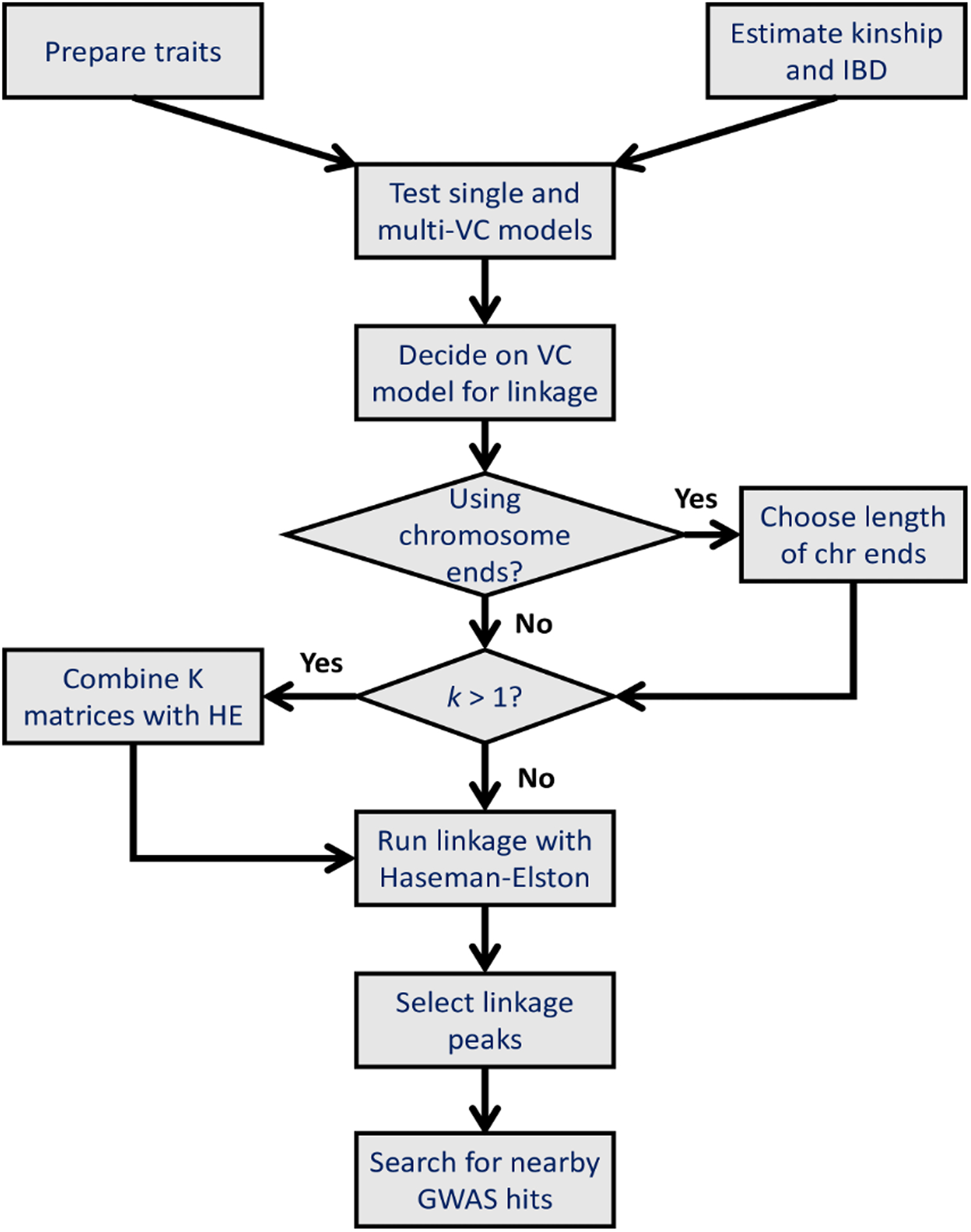
A flow chart showing the basic steps for researchers to run Population Linkage on their own data.

Notation

First, we introduce relevant notation. Assume we have genotype information on n individuals, and values for a quantitative trait, y. For each pair of individuals, i, j, their relatedness can be summarized by their kinship ϕ_ij, which is the probability that two randomly sampled alleles (one from each individual) are identical-by-descent (IBD). The full kinship matrix for all n(n − 1)/2 pairs of individuals is denoted as Φ. Two alternate summaries of the relationships between individuals include p_ij, the total proportion of DNA that is shared in IBD segments, and c_ijl, the total proportion of chromosome ends that are IBD in the first and last l megabases of each chromosome. These two additional summaries are important in ensuring calibration of our method as they enable us to cope with biases of population-based IBD estimates. We denote the full matrices of p_ij and c_ijl as P, and C_l, respectively. The full set of IBD segments are contained in S, where each element indicates the IBD status (1 or 2) and start and end position of the segment for a pair of individuals. The IBD status (0, 1, or 2) for individuals i and j at marker m can also be indicated as d_ijm, with the full matrix of all individuals’ IBD sharing at marker m as D_m.

The Data

The first step for Population Linkage is to prepare the input data. These consist of quantitative trait values from the cohort of interest and estimates of genetic relationships and allelic segregation (in the form of IBD estimates) between all pairs of individuals.

Traits

We prepare raw trait values y* for analysis by regressing on relevant covariates like age, sex, medication usage, and principal components, and then inverse-normalizing the residuals. This approach has the benefit of reducing the effect of extreme observations and will be helpful for obtaining a cross product yy^T that does not depend on the mean and variance of y*.

IBD segments

To estimate the set of all autosomal IBD segments S in our cohort, we used a particularly fast strategy for detecting these segments, implemented in the software package KING with the - ibdseg option (Young et al., 2022). From $\widehat{S}$, we calculate the matrix ${\widehat{D}}_m$ at the unique endpoints of all IBD segments in $\widehat{S}$ where there is a change in IBD status.

Proportion of IBD

From the collection of estimated autosomal IBD segments $\widehat{S}$ we calculate the genome-wide proportion $\widehat{P}$ of genetic material estimated to be shared IBD between each pair of individuals. $\widehat{P}$ is preferred over pedigree-calculated kinship in this context as a measure of genome-wide genetic similarity since pedigree information can be absent, incomplete, or incorrect, and actual realized IBD sharing in some instances diverges from theoretical expectations by a large amount (Thomson & McWhirter, 2017; Wang et al., 2017).

Kinship

A single statistic for genome-wide genetic similarity between pairs of individuals can fail to capture all the subtleties and nuances that exist in genetic relationships. One challenge presented by $\widehat{P}$ is that it is biased downward for distant relatives since the above method for estimating S does not consider IBD segments less than 2.5 Mb or 64 markers in length. For this reason, we also use the genotype-based kinship estimator $\widehat{\Phi }$ implemented in the KING software package (Manichaikul et al., 2010). This estimator is computationally efficient even with tens of thousands of individuals. In addition, it does not depend on allele frequencies and is robust in cohorts with population structure.

Proportion of IBD chromosome ends

There are additional challenges to estimating IBD segments at the ends of chromosomes. The end of each chromosome physically truncates the length of IBD segments, commercial genotyping arrays typically have lower marker density near chromosome ends, and the higher recombination rate in telomeres results in shorter IBD segments. These factors all lead to downward bias in ${\widehat{D}}_m$ toward the ends of chromosomes (Young et al., 2022), and importantly, the shared segments that can be identified tend to be concentrated in closer relatives who often have more similar trait values because of shared non-genetic but familial factors.

For these reasons, for all pairs of individuals we estimate C_ijl, the proportion of chromosome ends (of length l) that contain an IBD segment between individuals i and j. ${\widehat{C}}_{ijl}$ is the sum of the highest observed IBD status in the first and last l Mb of each chromosome in $\widehat{S}$ between individuals i and j, divided by twice the number of diploid chromosomes.

Statistical model

We begin this section by describing our framework for variance-components estimation and linkage analysis using cross-product Haseman-Elston regression.

Variance-Components model

For a model with k variance components for additive genetic effects, ${\sigma }_{{\mathit{\text{K}}}_1}^2,\dots ,{\sigma }_{{\mathit{\text{K}}}_{\mathit{\text{k}}}}^2$, we model trait variance in the following way:

$$var\left(\mathit{y}\right)={\sum }_{a=1}^k{K}_a{\sigma }_{{\mathit{\text{K}}}_a}^2+I{\sigma }_e^2$$ (Equation 1)

where K_a is a matrix of genetic relationships that has been centered so all rows and columns sum to 0 and scaled by the mean of its diagonal terms, and I is an n-by-n identity matrix. Since each K_a is scaled, ${\sigma }_{{\mathit{\text{K}}}_a}^2$ can also be interpreted as the proportion of variance explained (PVE) and ${\widehat{\sigma }}_e^2=1-{\sum }_{a=1}^{\mathit{\text{k}}}{\widehat{\sigma }}_{K_a}^2$ is the proportion of trait variance attributed to environmental effects and individual variability.

We obtain point estimates for ${\sigma }_{{\mathit{K}}_1}^2,\dots ,{\sigma }_{{\mathit{K}}_{\mathit{k}}}^2$ by cross-product Haseman-Elston regression using the following formulas from Zhou (2017):

$$\mathit{q}=\left(\begin{array}{c}{\mathit{y}}^T{K}_1-{\mathit{y}}^T\frac{n}{n-1}\\ ⋮\\ {\mathit{y}}^T{K}_k-{\mathit{y}}^T\frac{n}{n-1}\end{array}\right)\mathit{y}$$ (Equation 2)

$$S=\left(\begin{array}{ccc}tr\left(K_1{K}_1\right)& \cdots & tr\left(K_1{K}_k\right)\\ ⋮& \ddots & ⋮\\ tr\left(K_k{K}_1\right)& \cdots & tr\left(K_k{K}_k\right)\end{array}\right)-\frac{n^2}{n-1}$$ (Equation 3)

$${\widehat{\mathit{\sigma }}}^2=S^{-1}\mathit{q}$$ (Equation 4)

And the standard errors:

$$V\left(\mathit{q}\right)=2\left(\begin{array}{c}{\mathit{y}}^T{K}_1-{\mathit{y}}^T\frac{n}{n-1}\\ ⋮\\ {\mathit{y}}^T{K}_k-{\mathit{y}}^T\frac{n}{n-1}\end{array}\right)\left({\sum }_{a=1}^k{K}_a{\widehat{\sigma }}_{{\mathit{K}}_a}^2+I{\widehat{\sigma }}_e^2\right){\left(\begin{array}{c}{\mathit{y}}^T{K}_1-{\mathit{y}}^T\frac{n}{n-1}\\ ⋮\\ {\mathit{y}}^T{K}_k-{\mathit{y}}^T\frac{n}{n-1}\end{array}\right)}^T$$ (Equation 5)

$$V\left({\widehat{\mathit{\sigma }}}^2\right)=S^{-1}V\left(\mathit{q}\right)S^{-1}$$ (Equation 6)

$$SE\left({\widehat{\sigma }}_{{\mathit{K}}_a}^2\right)=\sqrt{V\left({\widehat{\sigma }}_{{\mathit{K}}_a}^2\right)},\forall a\in \left\{1,\dots ,k\right\}.$$ (Equation 7)

Equation 5 is an asymptotic approximation for V(q) and corresponds to an n-fold speedup (complexity O(k²n³) to O(k²n²)) for estimating the standard errors compared to using the expected information matrix (Zhou, 2017). Both the point estimates and standard errors are implemented in the GEMMA software package (Zhou, 2017; Zhou & Stephens, 2012).

VC linkage model

The full variance-components model for linkage analysis at a particular marker m is

$$\mathit{\text{var}}\left(\mathit{y}\right)=\tilde{\Phi }{\sigma }_{\tilde{\Phi }}^2+\tilde{P}{\sigma }_{\tilde{P}}^2+{\tilde{C}}_l{\sigma }_{{\tilde{C}}_l}^2+{\tilde{D}}_m{\sigma }_{{\tilde{D}}_m}^2+I{\sigma }_e^2.$$ (Equation 8)

The tilde over the matrices reflects that these are the centered and scaled versions of these matrices and not the original estimates. The fitting procedure for these models to obtain point estimates and standard errors of the variance components are the same as Equations 2–7. This fit must then be repeated at all marker locations m that will be tested for linkage.

After obtaining ${\widehat{\sigma }}_{{\tilde{D}}_m}^2$ and $SE\left({\widehat{\sigma }}_{{\tilde{D}}_m}^2\right)$, we test the null hypothesis of no linkage, $H_0: {\widehat{\sigma }}_{{\tilde{\mathbf{D}}}_m}^2=0$, against $H_1: {\widehat{\sigma }}_{{\tilde{\mathbf{D}}}_m}^2>0$. Since ${\widehat{\sigma }}_{{\tilde{D}}_m}^2/SE\left({\widehat{\sigma }}_{{\tilde{D}}_m}^2\right)$ is asymptotically normally distributed (Zhou, 2017) we compute its probability on the upper tail of the standard normal distribution to obtain a one-sided p-value for linkage. Logarithm of odds (LOD) is a traditional statistic for the strength of evidence for (or against) genetic linkage (Morton, 1955). For Population Linkage, we define

$$\text{LOD}={\log }_{10}L\left({\widehat{\sigma }}_{{\tilde{D}}_m}^2\right)/L\left({\sigma }_{{\tilde{D}}_m}^2=0\right),$$ (Equation 9)

and

$$L\left({\widehat{\sigma }}_{{\tilde{D}}_m}^2\right)=f\left(\raisebox{1ex}{${\widehat{\sigma }}_{{\tilde{D}}_m}^2$}\!\left/ \!\raisebox{-1ex}{$SE\left({\widehat{\sigma }}_{{\tilde{D}}_m}^2\right)$}\right.\right).$$ (Equation 10)

f here denotes the probability density function (PDF) of the standard normal distribution. From this likelihood, we can derive a simple equation for LOD score

$$\text{LOD=}\{\begin{array}{cc}0,& {\widehat{\sigma }}_{{\tilde{D}}_m}^2\le 0\\ \frac{(\raisebox{1ex}{${\widehat{\sigma }}_{{\tilde{D}}_m}^2$}\!\left/ \!\raisebox{-1ex}{$SE\left({\widehat{\sigma }}_{{\tilde{D}}_m}^2\right)$}\right.{)}^2}{2\log (10)},& {\widehat{\sigma }}_{{\tilde{D}}_m}^2>0\end{array}.$$ (Equation 11)

We set LOD = 0 when ${\widehat{\sigma }}_{{\tilde{D}}_m}^2\le 0$ because negative estimates for variance components do not constitute evidence for linkage. We use the established threshold of LOD > 3 for genome-wide significance which approximately corresponds to a one-sided p-value of 10⁻⁴ (Annunen et al., 1999; Risch, 1991).

Linkage analysis integration with GWAS

After completing the linkage analysis and calculating LOD scores across the genome, we report which loci show evidence of linkage with the trait of interest. Since the region over which LOD is greater than 3 can be large and span many loci tested with many small increases and decreases in LOD score, we report a specific site as a linkage peak if its LOD is greater than 3 and greater than the LOD scores of the two adjacent sites to the right and the two adjacent sites to the left. This peak marker then becomes the focus for follow up analyses.

Once GWAS results have been generated for the same data used in the linkage analysis, we extract all GWAS variants within 5 Mb of each linkage peak and choose the one with the smallest p-value for comparison. We chose to focus our search for GWAS variants within 5 Mb of linkage peaks because the 2.5 Mb minimum length to detect IBD segments limited the resolution of linkage peaks.

Computational approach

The previous sections describe how Population Linkage uses variance components estimated by Haseman-Elston regression to perform a genome-wide linkage analysis on population level data. Despite this improvement in scalability over full-likelihood linkage methods based on the Elston-Stewart (Elston & Stewart, 1971) or the Lander-Green (Lander & Green, 1987) algorithm, Population Linkage must still deal with several large n × n matrices as input and iterate over a dense marker map that can make the analysis time-consuming and challenging.

Our first strategy for improving the runtime of Population Linkage is to limit the number of sites tested to the unique endpoints of estimated IBD segments in $\widehat{S}$. We only fit Haseman-Elston regression and test for linkage at start and end coordinates in the set of $\widehat{S}$. This can reduce the number of sites tested to only those with distinct patterns of IBD sharing. To further limit the number of tests, one can optionally decide to test for linkage at fixed, evenly spaced intervals across the genome.

Our next strategy for improving the runtime of Population Linkage was to manage how our software processes input data. Because the large size of $\widehat{\Phi }$, $\widehat{P}$, ${\widehat{C}}_l$, and ${\widehat{D}}_m$, makes reading these inputs computationally burdensome, we try to minimize input and output by keeping quantities that will be re-used later in memory. We also calculate quantities that can be re-used across markers only once. For example, the first k − 1 terms in the q vector from Equation 2 and the first k − 1 rows and columns of the S matrix from Equation 3, and the intermediate calculation ${\mathit{y}}^T{K}_i-{\mathit{y}}^T\frac{n}{n-1}, i<k$ can be computed once and re-used across markers or analysis positions.

While high-performance computing systems can generally handle keeping the matrices $\tilde{\Phi }$, $\tilde{P}$, or ${\widehat{C}}_l$, in RAM for repeated use, when there are a large number of IBD segments in $\widehat{S}$ it may not be feasible to store all these in RAM to calculate ${\widehat{D}}_m$ and fit variance-components at every marker m. To remedy this issue, our process relies on sorting IBD segments and then gradually reading a small portion of IBD segment changes at a time, updating the matrix ${\widehat{D}}_m$, calculating linkage statistics, and then proceeding to load another small series of IBD segments after discarding previous ones that are no longer relevant.

We also simplify the linkage model with 4 variance components by fitting variance components for $\tilde{\Phi }$, $\tilde{P}$, and ${\tilde{C}}_l$ jointly without ${\widehat{D}}_m$ and then reweighting and combining into a single composite matrix

$$\tilde{K}=\left(\tilde{\Phi }{\sigma }_{\tilde{\Phi }}^2+\tilde{P}{\sigma }_{\tilde{P}}^2+{\tilde{C}}_l{\sigma }_{{\tilde{C}}_l}^2\right)\frac{1}{{\sigma }_{\tilde{\Phi }}^2+{\sigma }_{\tilde{P}}^2+{\sigma }_{{\tilde{C}}_l}^2}$$ (Equation 12)

to run linkage analysis with ${\widehat{D}}_m$, a 2-variance component model. This approach simplifies the linkage analysis because the matrices $\tilde{\Phi }$, $\tilde{P}$, and ${\tilde{C}}_l$ do not depend on m and their fit relative to one another only needs to be calculated once rather than repeated at all markers m. The rest of the analysis proceeds identically to the linkage analysis with the full model.

Implementation

The method we used for kinship and pairwise IBD estimation was implemented in KING versions 2.1.2 and higher (Chen et al., 2017). The Haseman-Elston regression in Equations 1–7 was implemented in GEMMA 0.96 (Zhou, 2017), which we modified to directly read in the output from KING, incorporate the computational enhancements described in this paper, and calculate LOD scores for linkage. This modified version and source code are available at https://github.com/gjmzajac/GEMMA-population-linkage.

Experimental data: SardiNIA

The SardiNIA project (Pilia et al., 2006) is an ongoing study of a population isolate in the Lanusei valley in the Italian island of Sardinia. This dataset comprises information on 6,602 individuals with genotype data at 18,754,911 autosomal variants that passed imputation quality filters (Nielsen et al., 2020). All samples were genotyped on commercial genotyping arrays and a subset of 3,445 of these samples were also sequenced and used to impute the remaining genotypes in the rest of the samples (Chiang et al., 2018; Gagliano et al., 2019; Pistis et al., 2015; Sidore et al., 2015). We estimated IBD and kinship in the full set of variants with KING 2.2. The dataset also included information on LDL cholesterol, HDL cholesterol, total cholesterol, and triglycerides together with covariates of sex, age and age². The SardiNIA study team also shared GWAS summary statistics generated by running EMMAX (Kang et al., 2010) with default settings on these same data.

Experimental data: HUNT

To see how well our method could scale to larger cohorts we chose to test for linkage in the HUNT study (Krokstad et al., 2013). Because of the multi-generational time scale and high participation rate in this sparsely populated region of Norway, the HUNT cohort contains a very large number of family relationships that can be inferred using the genetic data and used to test for genetic linkage. Genetic samples for 69,716 individuals were collected from the HUNT2 (1995–97) and HUNT3 (2006–08) population-based health surveys of all adults in the Nord-Trøndelag region in Norway (Brumpton et al., 2021). All samples were genotyped on a version of the IlluminaHumanCore-24 Exome array with custom content (Illumina, 2017). Genotypes at 359,432 autosomal variants phased with SHAPEIT2 (Delaneau et al., 2013) and imputed dosages at 45,453,131 autosomal variants (Brumpton et al., 2021) were available for Population Linkage and GWAS analyses. We estimated IBD and kinship with the 359,432 genotyped autosomal variants using KING 2.1.3.

As in SardiNIA, we focused our analyses on LDL cholesterol (estimated by the Friedewald formula), HDL cholesterol, total cholesterol, and triglycerides. We also used body mass index (BMI) as a control phenotype to help with model selection. As covariates, we used genetic principal components 1–4, genotyping batch, age at time of measurement, and sex.

To select a model for linkage analysis as described, we randomly sampled 25,000 HUNT participants and carried out a series of preliminary analyses with 1,000 equally spaced tests on a set of simulated trait values with no true linkage signals. We simulated a correlated phenotype for our cohort with covariance based on the genotype relatedness matrix (GRM) estimated by GEMMA 0.96 on the complete set of phased genotype data. After generating the linkage results and determining significant loci for each trait, we compared these with GWAS results generated using the SAIGE package (Zhou et al., 2018). In addition to these GWAS in the HUNT data, we also obtained summary statistics from the Global Lipids Genetics Consortium (GLGC) meta-analysis of these four lipid traits in 1.6 million individuals of European ancestry across 75 million variants (Graham et al., 2021).

Results

SardiNIA

We identified 44,006 putative relative pairs of 3rd degree or closer and a total of 316,729,132 IBD segments in the SardiNIA dataset. 97% of the individuals had at least one putative relative of 3rd degree or closer. All but 7 individuals shared at least one segment IBD with another individual. Table 1 summarizes the number of relative pairs, total and average number of IBD segments, and total and average length of IBD segments for each relationship type. The vast majority of estimated IBD segments (98.9%) were shared among distant relatives of 3rd degree or greater. These IBD segments would have been excluded in a linkage analysis that split the SardiNIA cohort into smaller pedigrees (Liu et al., 2008).

Table 1.

Relatedness and IBD sharing statistics in SardiNIA

Degree Relationship	N pairs	Tot. N IBD Segments	Avg. N IBD Segments per Pair	Tot. IBD Segment Length (Tb)	Avg. IBD Segment Length (Mb)
MZ Twins	16	1,455	91	0.1	59
Parent – Child	4,655	255,672	55	13	49
Full Siblings	5,442	906,470	167	15	16
2nd Degree	12,262	959,258	78	18	18
3rd Degree	21,631	1,386,018	64	17	12
> 3rd Degree	21,745,895	313,220,259	14	1,453	4.6

The number of pairs, total number of IBD segments estimated, average number of IBD segments per pair, total length of IBD segments estimated, and average length of IBD segments per pair by relationship type in SardiNIA, as estimated by KING 2.2.

We next fit single-variance component models using estimated kinship, genome-wide IBD proportion, and proportion of 1 Mb chromosome ends that were IBD for each of the four lipid traits: high-density lipoprotein cholesterol (HDL), low-density lipoprotein cholesterol (LDL), total cholesterol (TC), and triglycerides (TG) to calculate the proportion of variance explained (PVE) and genomic-control (GC) lambda values from linkage analyses of 1,000 equally spaced sites. The full results of these tests are reported in Table 2. Using the genome-wide IBD proportion matrix resulted in low GC lambda values (HDL 1.2, LDL 1.0, TC 1.1, TG 0.9) and visual inspection of the LOD plots (for example, see Figure 2) did not reveal any problems. We therefore used the genome-wide IBD proportion along with marker-specific IBD status to run linkage analysis of the four lipid traits at larger numbers of equally spaced sites and determine significant linkage peaks for SardiNIA.

Table 2.

Choice of fitting single variance components for linkage in SardiNIA

Pheno	N	VC	PVE (%)	GC Lambda
HDL	5,942	Kinship	40.1	2.74
HDL	5,942	IBD prop	36.7	1.16
HDL	5,942	Chr ends	38.5	4.44
LDL	5,937	Kinship	32.4	1.69
LDL	5,937	IBD prop	27.7	1.00
LDL	5,937	Chr ends	30.5	2.96
TC	5,937	Kinship	38.7	1.87
TC	5,937	IBD prop	33.7	1.10
TC	5,937	Chr ends	37.1	3.31
TG	5,905	Kinship	26.3	0.94
TG	5,905	IBD prop	20.8	0.91
TG	5,905	Chr ends	22.9	2.37

A table comparing the impact of different choices of single variance components on the proportion of variance explained (PVE) and genomic-control lambda (GC Lambda) in a linkage analysis of the phenotypes high-density lipoprotein cholesterol (HDL), low-density lipoprotein cholesterol (LDL), total cholesterol (TG), and triglycerides (TG) levels. “IBD prop” refers to the proportion of IBD shared genome-wide and “Chr ends” refers to average IBD sharing in the first and last Mb of each chromosome.

Figure 2. Overlap of LOD Scores for LDL with Known Regions.

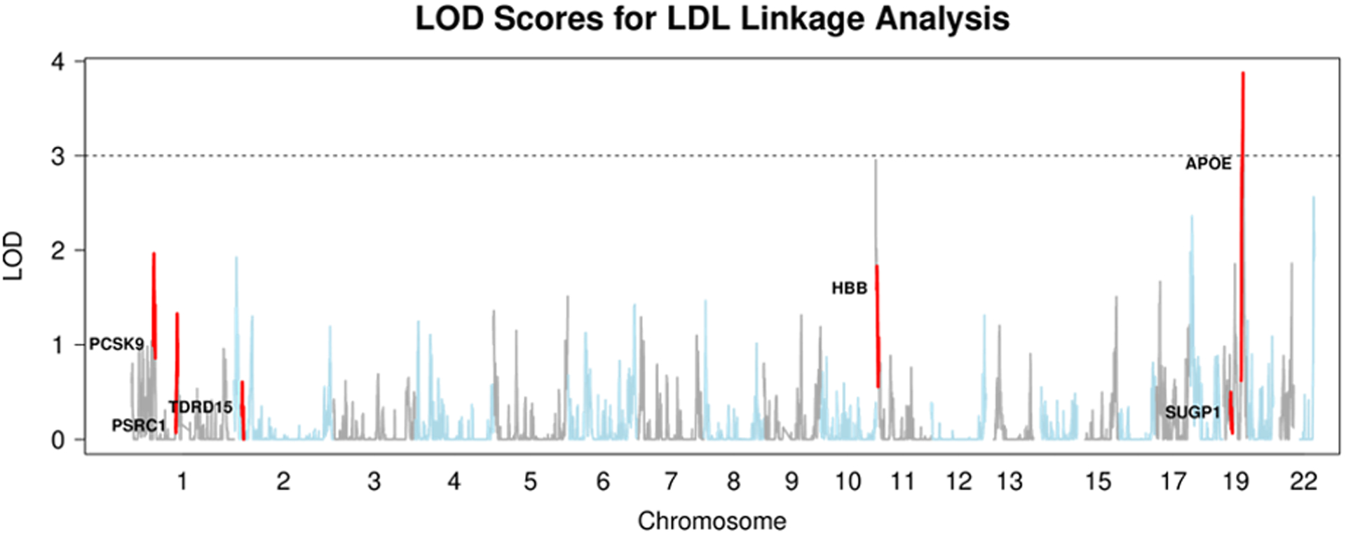
Above: LOD plot for the linkage analysis of LDL in SardiNIA. Below: GWAS of LDL in SardiNIA. Highlighted regions are the same in both plots.

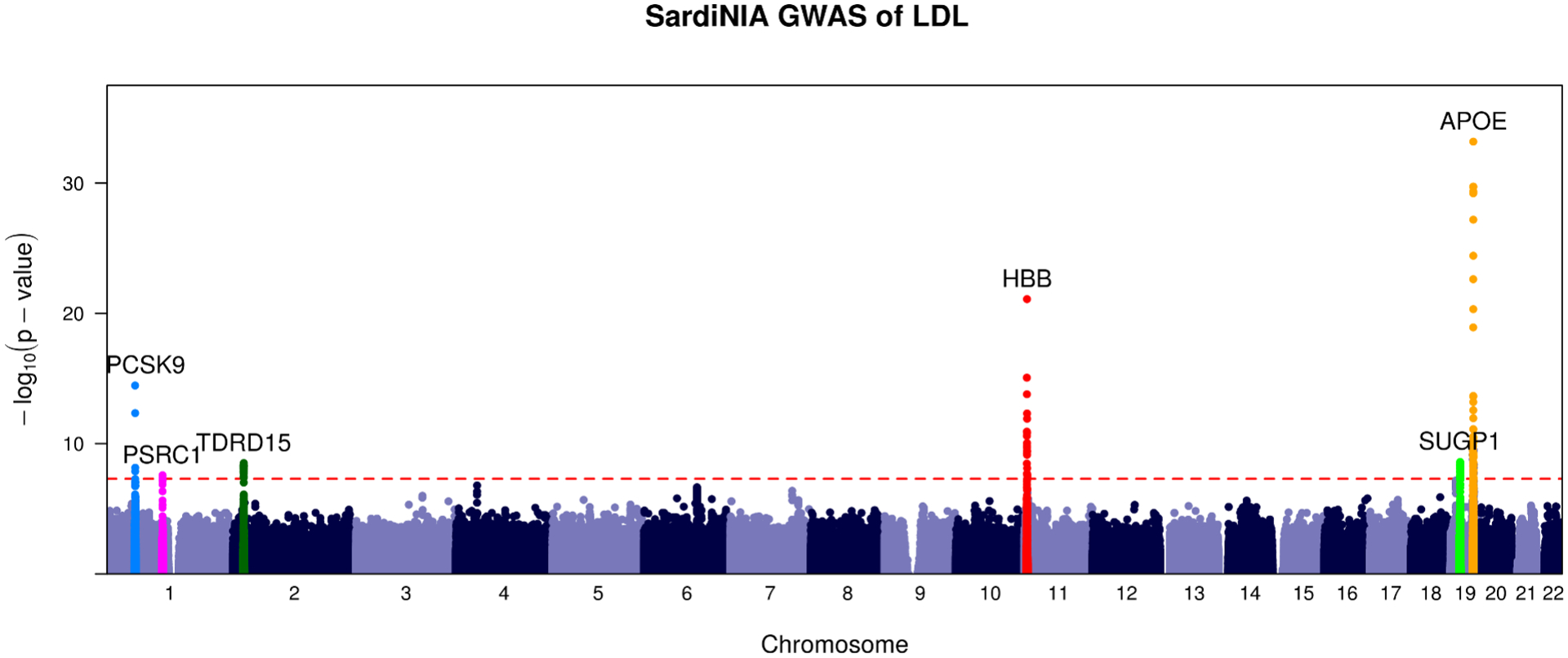
After calculating LOD scores for linkage in these 4 lipid traits, we had two significant peaks, one for the trait LDL and one for TC, both on chromosome 19 near the gene APOE (LDL LOD 3.9, PVE 5.0%; TC LOD 3.5, PVE 4.7%). These linkage peaks are reported in Table 3. The SardiNIA study (Sidore et al., 2015) previously associated the missense variants rs7412 and rs429358 in the gene APOE with variation in LDL and TC. rs429358 is well-known as a variant that disrupts APOE function in lipid transport and metabolism, influencing risk for Alzheimer’s disease, macular degeneration, and other traits (Jiang et al., 2008; Liutkeviciene et al., 2018). The original analysis showed that rs7412 and rs429358 were independent signals for both LDL and TC, with R² values of 2.4% and 0.8% for LDL and 1.7% and 0.5% for TC. Our linkage analysis estimated that IBD sharing in the APOE locus explained 5.0% of the variance in LDL and 4.7% for TC. This suggests that our linkage test captured the effects of both these variants and additional genetic variation in the region that influences LDL and TC levels that remains undetected through GWAS.

Table 3.

Linkage peaks in SardiNIA (19M SNPs) at different numbers of markers tested

Sites Tested	Trait	Gene	Chr	Pos	PVE (%)	LOD
1,000	LDL	APOE	19	47,471,344	4.8	3.54
	TC	APOE	19	47,471,344	4.3	3.05
5,000	LDL	APOE	19	48,030,170	4.9	3.74
	TC	APOE	19	48,030,170	4.7	3.46
10,000	LDL	APOE	19	48,030,170	4.9	3.74
	TC	APOE	19	48,287,640	4.8	3.49
20,000	LDL	APOE	19	47,880,669	5.0	3.88
	TC	APOE	19	47,880,669	4.7	3.54

Table of all linkage peaks with LOD > 3 in SardiNIA. The proportion of variance explained (PVE) and LOD for linkage, are reported at 1,000, 5,000, 10,000, and 20,000 equally spaced linkage tests. IBD estimates are from KING 2.2.

Our ability to observe this linkage signal for LDL and TC near APOE was not impacted by limiting the number of equally-spaced sites tested to 1,000, 5,000, 10,000, or 20,000 equally spaced genetic markers, with our method yielding LOD > 3 in each analysis (Table 3). While the number of sites tested impacted the largest observed LOD score in the region, calculating LOD scores at only 1,000 markers in order to improve runtime was sufficient to detect the strongest linkage signals present. This result is consistent with previous findings that only a few thousand loci needed to be tested in a genome-wide linkage scan of dense SNP genotypes (Matise et al., 2003).

Our linkage analysis successfully replicated the strongest GWAS signal for LDL in the gene APOE and showed elevated LOD scores near other GWAS peaks in HBB, PCSK9, and other genes (Figure 2). This result indicates that Population Linkage captures genetic effects in known lipid genes beyond APOE and that rerunning this analysis with a larger sample size might yield additional verifiable linkage peaks with LOD > 3.

HUNT

We estimated 451,864 relative pairs of 3rd degree or closer and a total of 6,867,367,662 IBD segments in the HUNT dataset. 93% of the individuals had at least one relative of 3rd degree or closer. The IBD estimates resulted in a total of 279,100 unique IBD segment endpoints. Table 4 gives a summary of the number of pairs of parent-offspring, full sibling, 2nd degree, 3rd degree, and more distant relationships, with the average and total number and length of estimated IBD segments in these relationship types. The vast majority (99.6%) of estimated IBD segments were in more distant relatives of 3rd degree or greater.

Table 4.

Relatedness and IBD sharing statistics in HUNT

Degree Relationship	N pairs	Tot. N IBD Segments	Avg. N IBD Segments	Tot. IBD Segment Length (Tb)	Avg. IBD Segment Length (Mb)
Parent – Child	47,113	2,105,385	45	126	60
Full Siblings	35,888	5,408,791	151	96	18
2nd Degree	117,478	7,639,166	65	163	21
3rd Degree	251,385	13,137,812	52	187	14
> 3rd Degree	2,429,673,606	6,839,076,508	2.8	31,939	4.7

The number of pairs, total number of IBD segments estimated, average number of IBD segments per pair, total length of IBD segments estimated, and average length of IBD segments per pair by relationship type in HUNT, as estimated by KING 2.1.3.

A preliminary linkage analysis of the null simulated phenotype with genome-wide IBD proportion revealed severe inflation in the test statistics at the ends of chromosomes (Figure 3, top) where IBD estimates were significantly biased toward close relatives (Figure 3, bottom). A diagnostic plot revealed an almost perfect correlation between this increased kinship of relatives IBD at the ends of chromosomes with the estimated proportion of variance explained (PVE) (Pearson’s correlation 0.99, Figure 4), driving up the LOD scores in those regions. Linkage analysis of LDL, body mass index (BMI), and the simulated phenotype with different choices of variance components in a randomly sampled subset of 25,000 samples revealed that simultaneously using estimated kinship, genome-wide IBD proportion, and IBD in 0.5 Mb chromosome ends resulted in GC lambda values near 1 (1.06 LDL, 1.15 BMI, 0.91 Simulation, Table 5, Table 6, Table 7). Reweighting and combining estimated kinship, IBD proportion, and IBD in 0.5 Mb chromosome ends into a single composite matrix resulted in z-scores for linkage that were almost perfectly correlated (r > 0.999 for LDL, BMI, and simulated trait) and LOD scores that were, on average, 0.0103, 0.0098, and 0.0124 lower for LDL, BMI, and the simulated trait, respectively. We concluded that using the combined matrix would adequately control for inflation at a negligible cost in statistical power while achieving similar runtime to the preliminary linkage analysis with only the genome-wide IBD proportion.

Figure 3. HUNT inflation example.

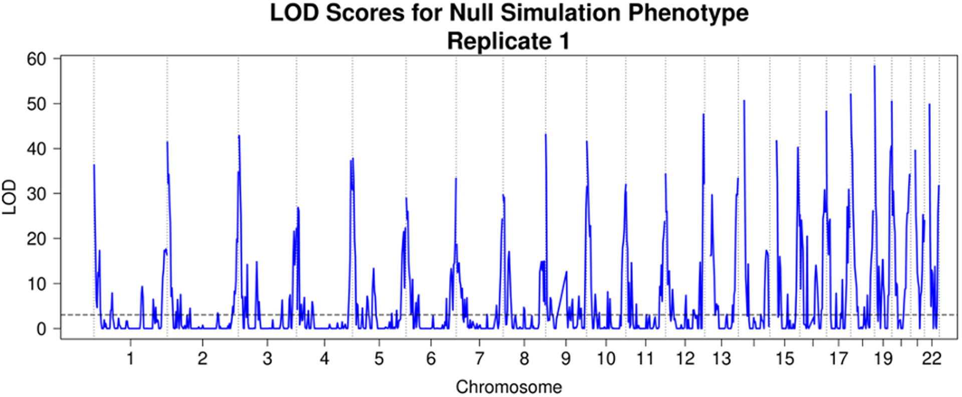
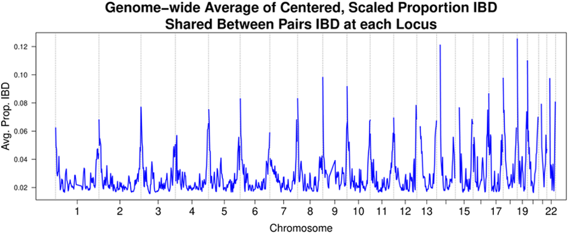
Above: LOD plot from linkage analysis of the null simulated phenotype across 69,716 HUNT samples, using genome-wide pairwise IBD proportion and region-specific IBD sharing as variance components. Below: The average kinship values for individuals IBD across the genome. The phenotype below is LDL (n = 67,429) so 2,287 samples in the simulation above do not appear in the plot below but otherwise the plots would be identical since the values of kinship and estimated IBD status at each marker do not depend on the phenotype.

Figure 4. Proportion of variance explained vs mean kinship of IBD pairs.

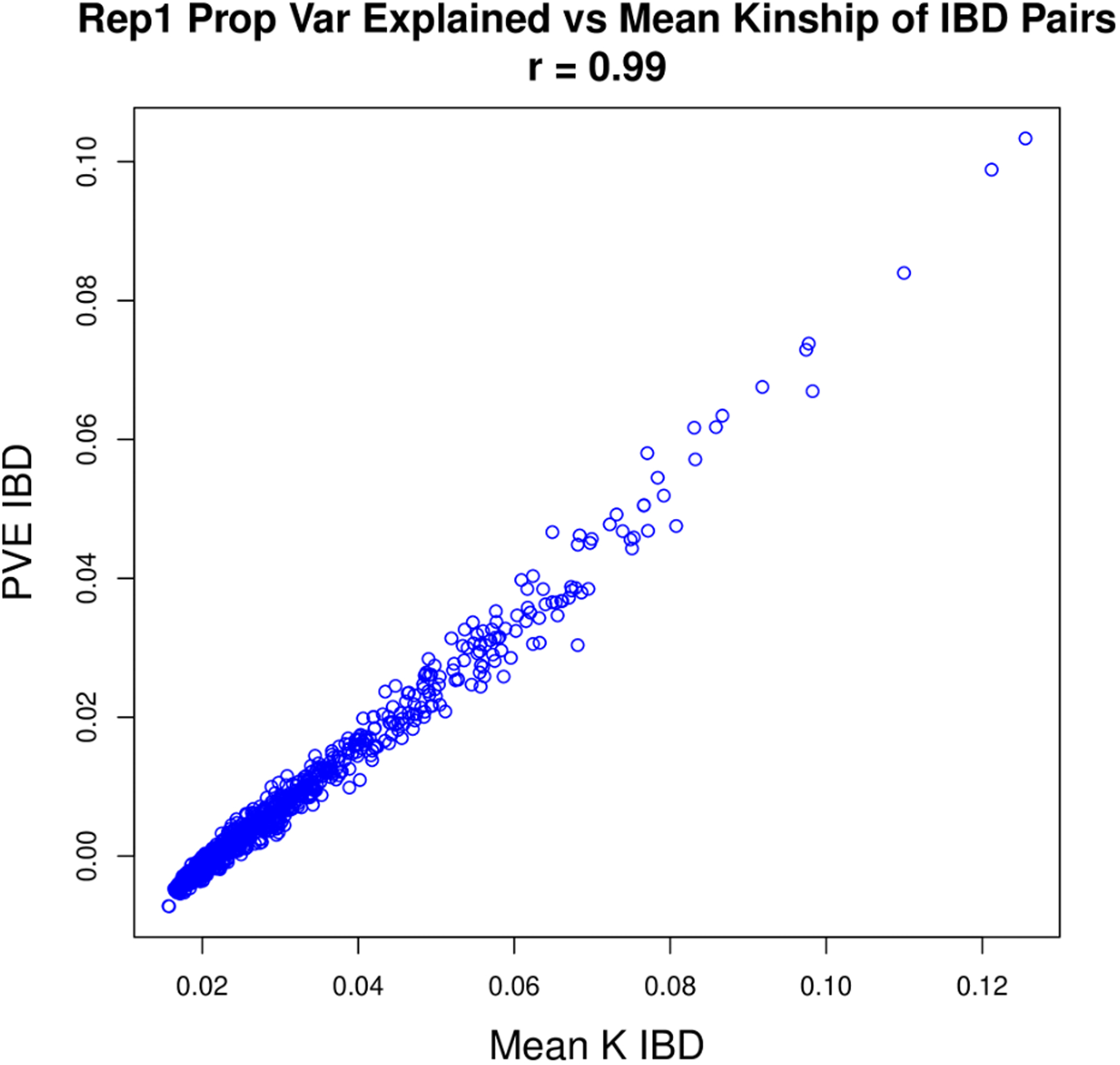
The estimated proportion of variance explained by IBD sharing at 1,000 sites from a linkage analysis of the HUNT null simulation phenotype plotted against the average kinship values for individuals IBD at each locus tested.

Table 5.

Choice of fitting single variance components for linkage in HUNT

Pheno	VC	PVE (%)	GC Lambda
BMI	Kinship	24.0	8.29
BMI	IBD prop	17.3	2.33
BMI	Chr ends	37.0	5.95
LDL	Kinship	30.0	20.29
LDL	IBD prop	26.0	2.73
LDL	Chr ends	50.2	12.61
Simulation	Kinship	62.8	3.62
Simulation	IBD prop	32.9	3.74
Simulation	Chr ends	68.8	15.83

A table comparing the impact of different choices of single variance components on the proportion of variance explained (PVE) and genomic-control lambda (GC Lambda) in a linkage analysis of the phenotypes LDL, BMI, and the null simulation. All results are from the random n=25,000 subset. “IBD prop” refers to the proportion of IBD shared genome-wide and “Chr ends” refers to average IBD sharing in the first and last Mb of each chromosome.

Table 6.

Choice of fitting multiple variance components for linkage

Pheno	VCs	Kinship PVE (%)	IBD prop PVE (%)	Chr ends PVE (%)	Total PVE (%)	GC
BMI	Kinship, IBD prop	20.0	8.1		28.1	1.49
BMI	Kinship, Chr ends	18.6		18.4	37.0	2.70
BMI	IBD prop, Chr ends		8.7	26.8	35.5	1.34
BMI	Kinship, IBD prop, Chr ends	17.7	4.7	13.8	36.2	1.15
LDL	Kinship, IBD prop	22.3	15.7		38.0	1.54
LDL	Kinship, Chr ends	21.7		28.5	50.3	6.56
LDL	IBD prop, Chr ends		15.8	31.6	47.4	1.29
LDL	Kinship, IBD prop, Chr ends	19.3	11.5	17.4	48.2	1.06
Sim	Kinship, IBD prop	60.4	5.0		65.4	0.99
Sim	Kinship, Chr ends	60.3		8.6	68.9	1.95
Sim	IBD prop, Chr ends		17.2	48.7	65.8	1.41
Sim	Kinship, IBD prop, Chr ends	59.6	3.8	4.9	68.3	0.91

A table comparing the impact of different combinations of variance components on the proportion of variance explained (PVE) and genomic-control lambda (GC) in a linkage analysis of the phenotypes LDL, BMI, and the null simulation. All results are from the random n=25,000 subset. “IBD prop” refers to the proportion of IBD shared genome-wide and “Chr ends” refers to average IBD sharing in the first and last Mb of each chromosome.

Table 7.

Choice of length of chromosome ends extracted

Mb Extracted	LDL PVE (%)	LDL GC	BMI PVE (%)	BMI GC	Sim PVE (%)	Sim GC
0.05	48.62	1.0477	36.47	1.1605	68.84	0.8991
0.1	48.67	1.0476	36.49	1.1573	68.80	0.8976
0.2	48.66	1.0478	36.45	1.1607	68.75	0.8958
0.3	48.58	1.0427	36.61	1.1255	68.68	0.8993
0.4	48.61	1.0432	36.66	1.1194	68.46	0.9090
0.5	48.35	1.0523	36.37	1.1306	68.34	0.9145
1	47.78	1.0536	35.87	1.1476	67.80	0.9221
2	46.54	1.0750	34.42	1.1861	67.48	0.9191
3	44.90	1.1712	33.29	1.2260	66.05	0.9760
4	43.48	1.1614	32.46	1.2356	65.52	0.9878
5	42.51	1.1670	31.52	1.2584	64.87	1.0380

A table comparing the impact of different choices of chromosome length extracted on the proportion of variance explained (PVE) by kinship, proportion of IBD shared, and average IBD sharing at the ends of chromosomes fit as a combined matrix and genomic-control lambda (GC) in a linkage analysis of the phenotypes LDL, BMI, and the null simulation. All results are from the random n=25,000 subset.

Once we had decided on this model with estimated kinship, genome-wide IBD proportion and IBD sharing at the ends of chromosomes, we proceeded to run linkage analysis on the 4 lipid traits (HDL, LDL, TC, and TG) at the full sample size. The sample sizes of our traits ranged from 67,429 for LDL to 69,479 for TG. Running each trait on one CPU core used an average of 133 GB RAM over 11 hours, 35 minutes for reweighting and combining matrices and 81 GB RAM over 11 days, 20 hours for linkage analysis.

We observed a total of 25 significant linkage peaks with LOD > 3 across 19 distinct loci for the four traits. HDL had 7 significant linkage peaks (Figure 5), LDL 9 (Figure 6), TC 7 (Figure 7), and TG 2 (Figure 8). All these peaks and supporting GWAS evidence for them are reported in Table 8. The majority of our significant linkage peaks were in established lipid loci that were easily replicated by our GWAS of genotyped and imputed HUNT variants and the GLGC meta-analysis. Our strongest signals were between the trait LDL and the region of chromosome 19 near the gene APOE (LOD 29.3, PVE 4.0%) and HDL and the region of chromosome 16 near the gene CETP (LOD 30.2, PVE 4.3%) both well known genes for lipid regulation (Freeman & Remaley, 2016) and were supported in the HUNT GWAS of genotyped variants, imputed variants, and the GLGC meta-analysis (Table 8).

Figure 5. HUNT HDL LOD Scores.

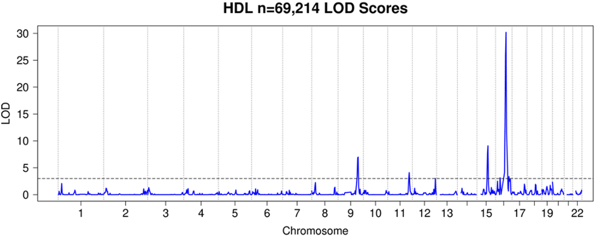
LOD plot from linkage analysis of HDL cholesterol levels from HUNT.

Figure 6. HUNT LDL LOD Scores.

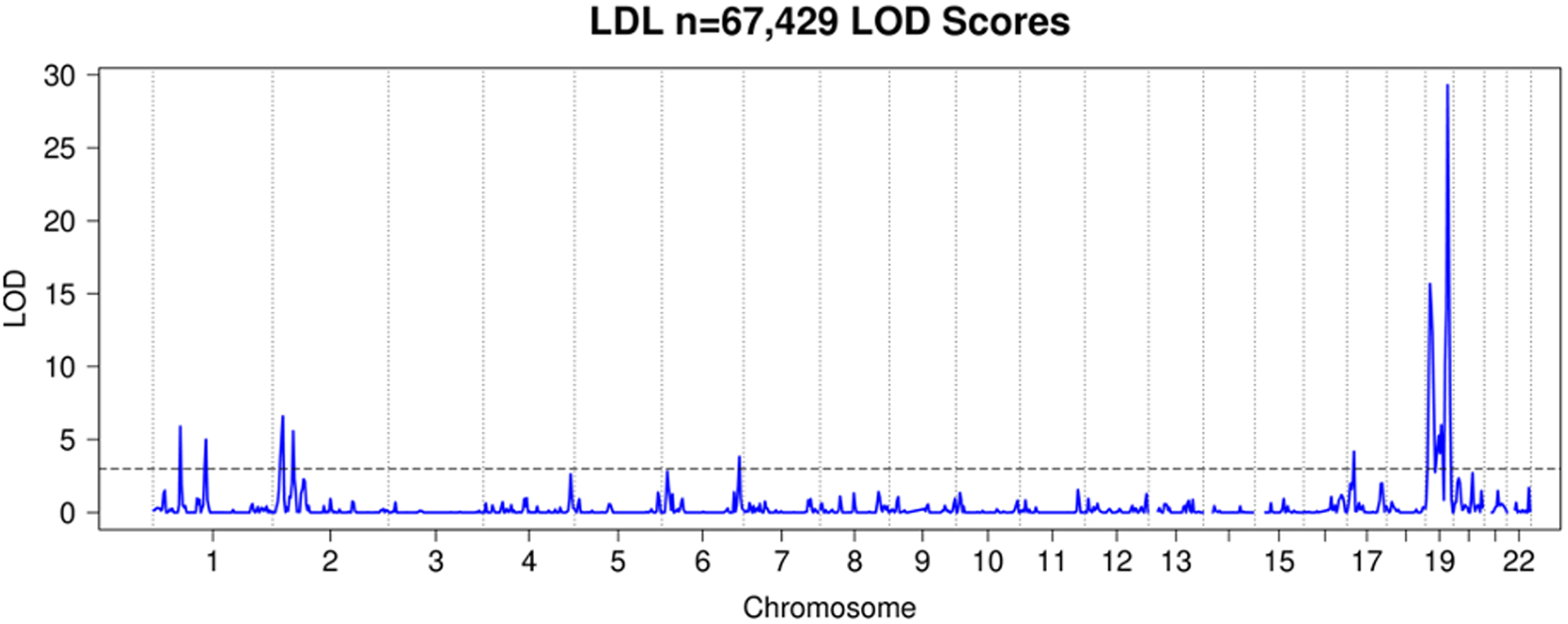
LOD plot from linkage analysis of LDL cholesterol levels from HUNT.

Figure 7. HUNT Total Cholesterol LOD Scores.

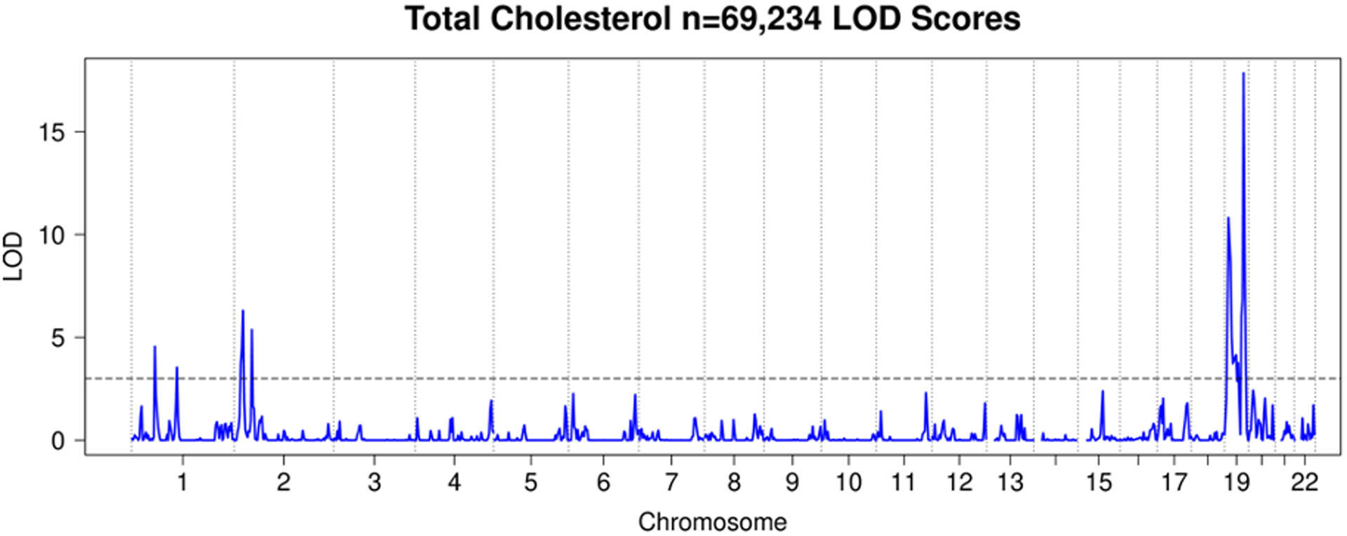
LOD plot from linkage analysis of TC levels from HUNT.

Figure 8. HUNT Triglycerides LOD Scores.

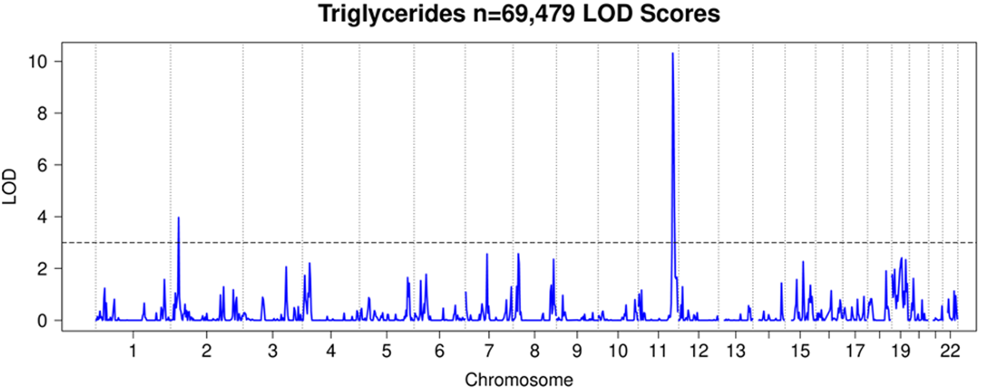
LOD plot from linkage analysis of TG levels from HUNT.

Table 8.

HUNT Linkage peaks

Trait	N	Chr:Mb	PVE IBD (%)	LOD	Geno p-value	Imputed p-value	GLGC p-value	Top SNP rsid	Top SNP Gene
HDL	69,214	9:110	1.18	7.0	3.9×10−61	3.7×10−61	1.3×10−420	rs2740488	ABCA1
HDL	69,214	11:118	0.60	4.1	4.8×10−30	4.8×10−30	1.4×10−637	rs964184	ZNF259
HDL	69,214	12:126	0.89	3.0	1.9×10−18	3.0×10−30	5.6×10−188	rs61941677	SCARB1
HDL	69,214	15:61	1.20	9.1	4.1×10−66	6.1×10−67	2.3×10−1162	rs261290	ALDH1A2
HDL	69,214	16:25	0.82	3.1	1.7×10−7	1.1×10−7	8.3×10−13	rs9938120	GPR139
HDL	69,214	16:58	4.26	30.2	1.6×10−225	1.1×10−234	2.2×10−5270	rs183130	CETP
HDL	69,214	16:74	0.54	3.4	6.4×10−6	1.5×10−42	9.2×10−46	rs571298027	CDH1
LDL	67,429	1:57	0.85	5.9	5.3×10−72	2.8×10−70	5.2×10−1390	rs11591147	PCSK9
LDL	67,429	1:110	0.81	5.0	1.5×10−46	1.2×10−46	4.7×10−1726	rs12740374	CELSR2
LDL	67,429	2:22	0.59	6.6	2.3×10−51	3.0×10−48	1.3×10−927	rs934197	APOB
LDL	67,429	2:43	0.79	5.6	6.0×10−35	5.1×10−35	1.4×10−470	rs4299376	ABCG8
LDL	67,429	6:162	0.89	3.8	9.8×10−13	5.3×10−28	5.5×10−377	rs10455872	LPA
LDL	67,429	17:15	0.55	4.2	3.4×10−4	9.4×10−8	6.4×10−13	rs28811342	LLGL1
LDL	67,429	19:10	1.19	15.7	1.8×10−86	2.2×10−88	1.4×10−2108	rs73015024	LDLR
LDL	67,429	19:33	0.83	6.0	5.0×10−4	3.6×10−9	3.3×10−12	rs147791730	CEBPG
LDL	67,429	19:47	4.05	29.3	0*	0*	5.6×10−8411	rs7412	APOE
TC	69,234	1:57	0.70	4.6	3.8×10−62	4.4×10−61	1.5×10−1119	rs11591147	PCSK9
TC	69,234	1:110	0.62	3.5	1.5×10−33	1.5×10−33	9.0×10−1298	rs12740374	CELSR2
TC	69,234	2:22	0.59	6.3	1.7×10−39	1.1×10−36	2.8×10−781	rs934197	APOB
TC	69,234	2:43	0.73	5.4	1.4×10−33	1.1×10−33	8.6×10−436	rs4299376	ABCG8
TC	69,234	19:10	0.91	10.8	1.2×10−69	4.2×10−70	1.0×10−1679	rs73015024	LDLR
TC	69,234	19:29	0.88	4.1	5.2×10−4	6.8×10−9	1.1×10−7	rs62108075	AC005307.3
TC	69,234	19:47	2.70	17.9	0*	0*	8.3×10−4123	rs7412	APOE
TG	69,479	2:27	0.35	4.0	4.5×10−30	1.4×10−29	6.6×10−1357	rs1260326	GCKR
TG	69,479	11:116	1.21	10.3	1.4×10−99	1.4×10−99	2.5×10−3336	rs964184	ZNF259

Table of all linkage peaks with LOD > 3 in HUNT. The PVE and LOD are from our linkage analysis. The smallest observed p-values within 5 Mb of each linkage peak from our GWAS of genotyped variants in HUNT, our GWAS of imputed variants in HUNT, and the GLGC meta-analysis are reported in the table. The rs ids and gene names in the table refer to the SNP with the smallest of these p-values for each linkage peak.

^*P-values of 0 are the result of underflow in the software used.

In addition to confirming known lipid genes, it was of interest to know where Population Linkage could provide additional insights beyond GWAS. There were 5 peaks with LOD > 3 which were not replicated at genome-wide significance in the HUNT GWAS of 359,432 genotyped variants. All of them were replicated in either the HUNT GWAS of imputed variants or the GLGC meta-analysis (Table 8). Since these 5 peaks did not have a genome-wide significant variant among single-variant tests of 359,432 genotyped variants that were used in the linkage analysis but were confirmed in either the HUNT GWAS of imputed variants or the GLGC meta-analysis, these results suggest that Population Linkage is able to detect linkage signals in ungenotyped variants.

Discussion

In this paper we introduced Population Linkage, which has enabled linkage analysis to be performed on larger sample sizes and in less time than ever before. We have demonstrated the feasibility of genome-wide linkage analysis on tens of thousands of individuals with hundreds of thousands of markers with our method, finding that this approach is able to replicate known associations in lipid traits and identify loci missed by GWAS of the same data. Sample relatedness is a nearly unavoidable situation in population or case-control cohorts of GWAS scale, prompting the development of an entire class of methods for linear-mixed-model GWAS to correct and control for the effect of sample relatedness (Kang et al., 2010; Kang et al., 2008; Zhou et al., 2018; Zhou & Stephens, 2012). By contrast, our method provides the opportunity to use this relatedness to map traits to genetic loci, often with greater variance explained in a region than the top associated SNP in GWAS. Additionally, because our method does not make any distributional assumptions about the phenotype and Haseman-Elston regression had been successfully extended to binary traits (Golan et al., 2014; Zeegers et al., 2003), we are hopeful that our method can be similarly adapted to perform linkage on binary traits with thousands of cases and controls.

In comparison to GWAS, Population Linkage offers potential advantages including estimation of the proportion of variance explained by all genetic variation in a region (rather than individual, observed variants), robust analysis in the presence of untyped genetic variation or population structure, and the ability to leverage cryptic relatedness in a data set. Despite the lower power of Population Linkage compared to GWAS at most loci, there are situations where we expect Population Linkage analysis will offer advantages – including for trait loci with substantial allelic heterogeneity. To illustrate, we highlight the relationship between breast cancer and BRCA1. Variation in BRCA1 has been identified as a risk factor for breast cancer in many linkage studies (Easton et al., 1993; Hall et al., 1990; Miki et al., 1994) but as of July 2022 there are still no GWAS reporting significant associations between breast cancer and BRCA1 (Buniello et al., 2019). The capacity of Population Linkage to scale linkage analysis to larger data with more loosely related individuals offers additional potential to characterize these types of traits and loci with linkage analysis. Population Linkage scales better than methods that attempt to estimate IBD jointly (and more accurately!) across many individuals (see, e.g. Glazner and Thompson (2015)). While some power is lost by analyzing pairwise IBD rather than joint IBD shared across many individuals, pairwise IBD is a convenient choice for fitting in the variance-components model used here.

One of the purported benefits of linkage analysis over GWAS is the ability to test for linkage in untyped genetic variation, as long as IBD segments in the region can be identified. Our results for HDL, LDL, and TC from the HUNT study support this claim since we observed 5 linkage signals with LOD > 3 where the GWAS of genotyped variants had no nearby genome-wide significant loci but GWAS with additional variants and/or samples did. In addition, our results for linkage in the APOE region in the SardiNIA study show how a test for linkage, even at a single marker, can capture the effects of multiple variants in the region that influence LDL levels. Since the inclusion of an individual SNP has little effect on the IBD estimates calculated in a region, this feature of linkage analysis would extend to capturing the effects of ungenotyped variants that influence the trait as well. Significant linkage findings can then give impetus to additional targeted sequencing, methylation analyses, and other functional characterization in purported linked regions to yield a more complete catalogue of variant effects.

This work opens new possibilities for how linkage analysis might be further applied and developed in the future. These could include incorporating new algorithms for fitting genetic variance components even more quickly (Hou et al., 2019; Pazokitoroudi et al., 2020), linkage analysis with shorter IBD segments at higher resolution via whole-genome sequencing data, or recent innovations in finding shorter IBD segments in distant, apparently unrelated, individuals (Delaneau et al., 2019). Most importantly, a seamless integration of variance components linkage analysis and GWAS into a joint mixed effects model can increase the power and utility of both. Such an approach can not only combine the signal from both linkage and association for a more powerful test to find additional novel associations, but also opens the possibility of testing a variant for association conditioned on the genetic background of individuals in a region. This can help to fine map causal variants in a region that shows evidence for association and further our understanding of how they impact biology and disease risk.

Data Availability Statement

SardiNIA project data are only available for sharing and collaborating on by request from the project leader, Francesco Cucca, Consiglio Nazionale delle Ricerche, Italy.

If interested in accessing HUNT data, you can find more information at https://www.ntnu.edu/hunt/data.

References

- Abecasis GR, Cherny SS, Cookson WO, & Cardon LR (2002). Merlin--rapid analysis of dense genetic maps using sparse gene flow trees. Nature Genetics, 30(1), 97–101. [DOI] [PubMed] [Google Scholar]
- Amos CI (1994). Robust variance-components approach for assessing genetic linkage in pedigrees. American Journal of Human Genetics, 54(3), 535–543. [PMC free article] [PubMed] [Google Scholar]
- Annunen S, Paassilta P, Lohiniva J, Perälä M, Pihlajamaa T, Karppinen J, … Ala-Kokko L (1999). An allele of COL9A2 associated with intervertebral disc disease. Science, 285(5426), 409–412. 10.1126/science.285.5426.409 [DOI] [PubMed] [Google Scholar]
- Blangero J, Williams JT, & Almasy L (2001). Variance component methods for detecting complex trait loci. Adv Genet, 42, 151–181. 10.1016/s0065-2660(01)42021-9 [DOI] [PubMed] [Google Scholar]
- Brumpton BM, Graham S, Surakka I, Skogholt AH, Løset M, Fritsche LG, … Willer CJ (2021). The HUNT Study: a population-based cohort for genetic research. medRxiv, 2021.2012.2023.21268305 10.1101/2021.12.23.21268305 [DOI] [PMC free article] [PubMed] [Google Scholar]
- Buniello A, MacArthur JAL, Cerezo M, Harris LW, Hayhurst J, Malangone C, … Parkinson H (2019). The NHGRI-EBI GWAS Catalog of published genome-wide association studies, targeted arrays and summary statistics 2019. Nucleic Acids Res, 47(D1), D1005–D1012. 10.1093/nar/gky1120 [DOI] [PMC free article] [PubMed] [Google Scholar]
- Chen GB (2014). Estimating heritability of complex traits from genome-wide association studies using IBS-based Haseman-Elston regression. Front Genet, 5, 107. 10.3389/fgene.2014.00107 [DOI] [PMC free article] [PubMed] [Google Scholar]
- Chen WM, Manichaikul A, Nguyen J, Onengut-Gumuscu S, & Rich SS (2017). Integrated inference that accurately identifies close relatives in > 1 million samples. Annual Meeting of the American Society of Human Genetics 2017, Orlando, FL. [Google Scholar]
- Chiang CWK, Marcus JH, Sidore C, Biddanda A, Al-Asadi H, Zoledziewska M, … Novembre J (2018). Genomic history of the Sardinian population. Nat Genet, 50(10), 1426–1434. 10.1038/s41588-018-0215-8 [DOI] [PMC free article] [PubMed] [Google Scholar]
- Day-Williams AG, Blangero J, Dyer TD, Lange K, & Sobel EM (2011). Linkage analysis without defined pedigrees. Genet Epidemiol, 35(5), 360–370. 10.1002/gepi.20584 [DOI] [PMC free article] [PubMed] [Google Scholar]
- Delaneau O, Zagury JF, & Marchini J (2013). Improved whole-chromosome phasing for disease and population genetic studies. Nat Methods, 10(1), 5–6. 10.1038/nmeth.2307 [DOI] [PubMed] [Google Scholar]
- Delaneau O, Zagury JF, Robinson MR, Marchini JL, & Dermitzakis ET (2019). Accurate, scalable and integrative haplotype estimation. Nat Commun, 10(1), 5436. 10.1038/s41467-019-13225-y [DOI] [PMC free article] [PubMed] [Google Scholar]
- Donnelly KP (1983). The probability that related individuals share some section of genome identical by descent. Theor Popul Biol, 23(1), 34–63. 10.1016/0040-5809(83)90004-7 [DOI] [PubMed] [Google Scholar]
- Easton DF, Bishop DT, Ford D, & Crockford GP (1993). Genetic linkage analysis in familial breast and ovarian cancer: results from 214 families. The Breast Cancer Linkage Consortium. Am J Hum Genet, 52(4), 678–701. [PMC free article] [PubMed] [Google Scholar]
- Elston RC, & Stewart J (1971). A general model for the genetic analysis of pedigree data. Hum Hered, 21(6), 523–542. 10.1159/000152448 [DOI] [PubMed] [Google Scholar]
- Evans DM, & Cardon LR (2004). Guidelines for genotyping in genomewide linkage studies: single-nucleotide-polymorphism maps versus microsatellite maps. Am J Hum Genet, 75(4), 687–692. 10.1086/424696 [DOI] [PMC free article] [PubMed] [Google Scholar]
- Freeman LA, & Remaley AT (2016). Chapter 6 - Discovery of High-Density Lipoprotein Gene Targets from Classical Genetics to Genome-Wide Association Studies. In Rodriguez-Oquendo A (Ed.), Translational Cardiometabolic Genomic Medicine (pp. 119–159). Academic Press. https://doi.org/ 10.1016/B978-0-12-799961-6.00006-8 [DOI] [Google Scholar]
- Gagliano SA, Sengupta S, Sidore C, Maschio A, Cucca F, Schlessinger D, & Abecasis GR (2019). Relative impact of indels versus SNPs on complex disease. Genet Epidemiol, 43(1), 112–117. 10.1002/gepi.22175 [DOI] [PMC free article] [PubMed] [Google Scholar]
- Georgi B, Craig D, Kember RL, Liu W, Lindquist I, Nasser S, … Bucan M (2014). Genomic view of bipolar disorder revealed by whole genome sequencing in a genetic isolate. PLoS Genet, 10(3), e1004229. 10.1371/journal.pgen.1004229 [DOI] [PMC free article] [PubMed] [Google Scholar]
- Glazner C, & Thompson E (2015). Pedigree-Free Descent-Based Gene Mapping from Population Samples. Hum Hered, 80(1), 21–35. 10.1159/000430841 [DOI] [PMC free article] [PubMed] [Google Scholar]
- Golan D, Lander ES, & Rosset S (2014). Measuring missing heritability: inferring the contribution of common variants. Proc Natl Acad Sci U S A, 111(49), E5272–5281. 10.1073/pnas.1419064111 [DOI] [PMC free article] [PubMed] [Google Scholar]
- Graham SE, Clarke SL, Wu KH, Kanoni S, Zajac GJM, Ramdas S, … Consortium*, G. L. G. (2021). The power of genetic diversity in genome-wide association studies of lipids. Nature, 600(7890), 675–679. 10.1038/s41586-021-04064-3 [DOI] [PMC free article] [PubMed] [Google Scholar]
- Hall JM, Lee MK, Newman B, Morrow JE, Anderson LA, Huey B, & King MC (1990). Linkage of early-onset familial breast cancer to chromosome 17q21. Science, 250(4988), 1684–1689. 10.1126/science.2270482 [DOI] [PubMed] [Google Scholar]
- Haseman JK, & Elston RC (1972). The investigation of linkage between a quantitative trait and a marker locus. Behav Genet, 2(1), 3–19. 10.1007/bf01066731 [DOI] [PubMed] [Google Scholar]
- Hodge SE, Hager VR, & Greenberg DA (2016). Using Linkage Analysis to Detect Gene-Gene Interactions. 2. Improved Reliability and Extension to More-Complex Models. PLoS One, 11(1), e0146240. 10.1371/journal.pone.0146240 [DOI] [PMC free article] [PubMed] [Google Scholar]
- Hou K, Burch KS, Majumdar A, Shi H, Mancuso N, Wu Y, … Pasaniuc B (2019). Accurate estimation of SNP-heritability from biobank-scale data irrespective of genetic architecture. Nat Genet, 51(8), 1244–1251. 10.1038/s41588-019-0465-0 [DOI] [PMC free article] [PubMed] [Google Scholar]
- Illumina. (2017). Infinium ® CoreExome- 24 v1.2 BeadChip. https://www.illumina.com/content/dam/illumina-marketing/documents/products/datasheets/datasheet_human_core_exome_beadchip.pdf.
- Jiang Q, Lee CY, Mandrekar S, Wilkinson B, Cramer P, Zelcer N, … Landreth GE (2008). ApoE promotes the proteolytic degradation of Abeta. Neuron, 58(5), 681–693. 10.1016/j.neuron.2008.04.010 [DOI] [PMC free article] [PubMed] [Google Scholar]
- Kang HM, Sul JH, Service SK, Zaitlen NA, Kong SY, Freimer NB, … Eskin E (2010). Variance component model to account for sample structure in genome-wide association studies. Nat Genet, 42(4), 348–354. 10.1038/ng.548 [DOI] [PMC free article] [PubMed] [Google Scholar]
- Kang HM, Zaitlen NA, Wade CM, Kirby A, Heckerman D, Daly MJ, & Eskin E (2008). Efficient control of population structure in model organism association mapping. Genetics, 178(3), 1709–1723. https://doi.org/178/3/1709 [pii] 10.1534/genetics.107.080101 [DOI] [PMC free article] [PubMed] [Google Scholar]
- Kathiresan S, Manning AK, Demissie S, D’Agostino RB, Surti A, Guiducci C, … Cupples LA (2007). A genome-wide association study for blood lipid phenotypes in the Framingham Heart Study. BMC Med Genet, 8 Suppl 1, S17. 10.1186/1471-2350-8-S1-S17 [DOI] [PMC free article] [PubMed] [Google Scholar]
- Krokstad S, Langhammer A, Hveem K, Holmen TL, Midthjell K, Stene TR, … Holmen J (2013). Cohort Profile: the HUNT Study, Norway. Int J Epidemiol, 42(4), 968–977. 10.1093/ije/dys095 [DOI] [PubMed] [Google Scholar]
- Lander ES, & Green P (1987). Construction of multilocus genetic linkage maps in humans. Proc Natl Acad Sci U S A, 84(8), 2363–2367. 10.1073/pnas.84.8.2363 [DOI] [PMC free article] [PubMed] [Google Scholar]
- Lange K, & Boehnke M (1983). Extensions to pedigree analysis. IV. Covariance components models for multivariate traits. American Journal of Medical Genetics, 14(3), 513–524. [DOI] [PubMed] [Google Scholar]
- Lange K, & Sobel E (1991). A random walk method for computing genetic location scores. Am J Hum Genet, 49(6), 1320–1334. [PMC free article] [PubMed] [Google Scholar]
- Liu F, Kirichenko A, Axenovich TI, van Duijn CM, & Aulchenko YS (2008). An approach for cutting large and complex pedigrees for linkage analysis. Eur J Hum Genet, 16(7), 854–860. 10.1038/ejhg.2008.24 [DOI] [PubMed] [Google Scholar]
- Liutkeviciene R, Vilkeviciute A, Smalinskiene A, Tamosiunas A, Petkeviciene J, Zaliuniene D, & Lesauskaite V (2018). The role of apolipoprotein E (rs7412 and rs429358) in age-related macular degeneration. Ophthalmic Genet, 39(4), 457–462. 10.1080/13816810.2018.1479429 [DOI] [PubMed] [Google Scholar]
- Manichaikul A, Mychaleckyj JC, Rich SS, Daly K, Sale M, & Chen WM (2010). Robust relationship inference in genome-wide association studies. Bioinformatics, 26(22), 2867–2873. 10.1093/bioinformatics/btq559 [DOI] [PMC free article] [PubMed] [Google Scholar]
- Matise TC, Sachidanandam R, Clark AG, Kruglyak L, Wijsman E, Kakol J, … Holden AL (2003). A 3.9-centimorgan-resolution human single-nucleotide polymorphism linkage map and screening set. Am J Hum Genet, 73(2), 271–284. 10.1086/377137 [DOI] [PMC free article] [PubMed] [Google Scholar]
- Miki Y, Swensen J, Shattuck-Eidens D, Futreal PA, Harshman K, Tavtigian S, … Ding W (1994). A strong candidate for the breast and ovarian cancer susceptibility gene BRCA1. Science, 266(5182), 66–71. 10.1126/science.7545954 [DOI] [PubMed] [Google Scholar]
- Minster RL, Sanders JL, Singh J, Kammerer CM, Barmada MM, Matteini AM, … Newman AB (2015). Genome-Wide Association Study and Linkage Analysis of the Healthy Aging Index. J Gerontol A Biol Sci Med Sci, 70(8), 1003–1008. 10.1093/gerona/glv006 [DOI] [PMC free article] [PubMed] [Google Scholar]
- Morton NE (1955). Sequential tests for the detection of linkage. Am J Hum Genet, 7(3), 277–318. [PMC free article] [PubMed] [Google Scholar]
- Mousavi N, Shleizer-Burko S, Yanicky R, & Gymrek M (2019). Profiling the genome-wide landscape of tandem repeat expansions. Nucleic Acids Res, 47(15), e90. 10.1093/nar/gkz501 [DOI] [PMC free article] [PubMed] [Google Scholar]
- Nielsen JB, Rom O, Surakka I, Graham SE, Zhou W, Roychowdhury T, … Hveem K (2020). Loss-of-function genomic variants highlight potential therapeutic targets for cardiovascular disease. Nat Commun, 11(1), 6417. 10.1038/s41467-020-20086-3 [DOI] [PMC free article] [PubMed] [Google Scholar]
- Oikkonen J, Huang Y, Onkamo P, Ukkola-Vuoti L, Raijas P, Karma K, … Järvelä I (2015). A genome-wide linkage and association study of musical aptitude identifies loci containing genes related to inner ear development and neurocognitive functions. Mol Psychiatry, 20(2), 275–282. 10.1038/mp.2014.8 [DOI] [PMC free article] [PubMed] [Google Scholar]
- Pazokitoroudi A, Wu Y, Burch KS, Hou K, Zhou A, Pasaniuc B, & Sankararaman S (2020). Efficient variance components analysis across millions of genomes. Nat Commun, 11(1), 4020. 10.1038/s41467-020-17576-9 [DOI] [PMC free article] [PubMed] [Google Scholar]
- Pilia G, Chen WM, Scuteri A, Orru M, Albai G, Dei M, … Schlessinger D (2006). Heritability of cardiovascular and personality traits in 6,148 Sardinians. PLoS Genet, 2(8), e132. https://doi.org/06-PLGE-RA-0086R2 [pii] 10.1371/journal.pgen.0020132 [DOI] [PMC free article] [PubMed] [Google Scholar]
- Pistis G, Porcu E, Vrieze SI, Sidore C, Steri M, Danjou F, … Sanna S (2015). Rare variant genotype imputation with thousands of study-specific whole-genome sequences: implications for cost-effective study designs. Eur J Hum Genet, 23(7), 975–983. 10.1038/ejhg.2014.216 [DOI] [PMC free article] [PubMed] [Google Scholar]
- Piven J, Vieland VJ, Parlier M, Thompson A, O’Conner I, Woodbury-Smith M, … Szatmari P (2013). A molecular genetic study of autism and related phenotypes in extended pedigrees. J Neurodev Disord, 5(1), 30. 10.1186/1866-1955-5-30 [DOI] [PMC free article] [PubMed] [Google Scholar]
- Risch N (1991). A note on multiple testing procedures in linkage analysis. Am J Hum Genet, 48(6), 1058–1064. [PMC free article] [PubMed] [Google Scholar]
- Sham PC, & Purcell S (2001). Equivalence between Haseman-Elston and variance-components linkage analyses for sib pairs. Am J Hum Genet, 68(6), 1527–1532. 10.1086/320593 [DOI] [PMC free article] [PubMed] [Google Scholar]
- Sham PC, Purcell S, Cherny SS, & Abecasis GR (2002). Powerful regression-based quantitative-trait linkage analysis of general pedigrees. American Journal of Human Genetics, 71(2), 238–253. [DOI] [PMC free article] [PubMed] [Google Scholar]
- Sidore C, Busonero F, Maschio A, Porcu E, Naitza S, Zoledziewska M, … Abecasis GR (2015). Genome sequencing elucidates Sardinian genetic architecture and augments association analyses for lipid and blood inflammatory markers. Nat Genet, 47(11), 1272–1281. 10.1038/ng.3368 [DOI] [PMC free article] [PubMed] [Google Scholar]
- Thompson EA (2019). Descent‐Based Gene Mapping in Pedigrees and Populations. Handbook of Statistical Genomics: Two Volume Set, 573–596. [Google Scholar]
- Thomson R, & McWhirter R (2017). Adjusting for Familial Relatedness in the Analysis of GWAS Data. Methods Mol Biol, 1526, 175–190. 10.1007/978-1-4939-6613-4_10 [DOI] [PubMed] [Google Scholar]
- Tong L, & Thompson E (2008). Multilocus lod scores in large pedigrees: combination of exact and approximate calculations. Hum Hered, 65(3), 142–153. 10.1159/000109731 [DOI] [PMC free article] [PubMed] [Google Scholar]
- Van Arendonk JA, Tier B, Bink MC, & Bovenhuis H (1998). Restricted maximum likelihood analysis of linkage between genetic markers and quantitative trait loci for a granddaughter design. J Dairy Sci, 81 Suppl 2, 76–84. 10.3168/jds.s0022-0302(98)70156-0 [DOI] [PubMed] [Google Scholar]
- Vieland VJ, Huang Y, Seok SC, Burian J, Catalyurek U, O’Connell J, … Valentine-Cooper W (2011). KELVIN: a software package for rigorous measurement of statistical evidence in human genetics. Hum Hered, 72(4), 276–288. 10.1159/000330634 [DOI] [PMC free article] [PubMed] [Google Scholar]
- Wang B, Sverdlov S, & Thompson E (2017). Efficient Estimation of Realized Kinship from Single Nucleotide Polymorphism Genotypes. Genetics, 205(3), 1063–1078. 10.1534/genetics.116.197004 [DOI] [PMC free article] [PubMed] [Google Scholar]
- Young AI, Nehzati SM, Benonisdottir S, Okbay A, Jayashankar H, Lee C, … Kong A (2022). Mendelian imputation of parental genotypes improves estimates of direct genetic effects. Nat Genet, 54(6), 897–905. 10.1038/s41588-022-01085-0 [DOI] [PMC free article] [PubMed] [Google Scholar]
- Zeegers MP, Rice JP, Rijsdijk FV, Abecasis GR, & Sham PC (2003). Regression-based sib pair linkage analysis for binary traits. Hum Hered, 55(2–3), 125–131. 10.1159/000072317 [DOI] [PubMed] [Google Scholar]
- Zhou W, Nielsen JB, Fritsche LG, Dey R, Gabrielsen ME, Wolford BN, … Lee S (2018). Efficiently controlling for case-control imbalance and sample relatedness in large-scale genetic association studies. Nat Genet, 50(9), 1335–1341. 10.1038/s41588-018-0184-y [DOI] [PMC free article] [PubMed] [Google Scholar]
- Zhou X (2017). A Unified Framework for Variance Component Estimation with Summary Statistics in Genome-Wide Association Studies. Ann Appl Stat, 11(4), 2027–2051. 10.1214/17-AOAS1052 [DOI] [PMC free article] [PubMed] [Google Scholar]
- Zhou X, & Stephens M (2012). Genome-wide efficient mixed-model analysis for association studies. Nature Genetics, 44(7), 821–824. 10.1038/ng.2310 [DOI] [PMC free article] [PubMed] [Google Scholar]
Associated Data
This section collects any data citations, data availability statements, or supplementary materials included in this article.